9.2. Utility Programs¶

orca_2aim	Produces WFN and WFX files suitable for AIM analysis
orca_2json	Converts information from the gbw-file into JSON files
orca_2mkl	Produces an ASCII file to be read by molekel, molden or other visualization programs
orca_asa	Calculates band shapes of absorption, fluorescence and resonance Raman spectra
orca_chelpg	Calculates electrostatic potential derived charges
orca_euler	Calculates Euler angles from `.property.txt` file
orca_exportbasis	Prints out any basis set in ORCA or GAMESS-US format
orca_fitpes	Fits potential energy curves of diatomics
orca_mapspc	Produces files for transfer into plotting programs
orca_mergefrag	Merges MO coefficients from two independent .gbw files
orca_pltvib	Produces files for the animation of vibrations
orca_pnmr	Calculates paramagnetic NMR shielding tensors
orca_vib	Calculates vibrational frequencies from a completed frequency run (also used for isotope shift calculations)
otool_gcp	Calculates Geometrical Counterpoise Correction (GCP)
otool_xtb	Allows using standalone xTB code from the Grimme lab with ORCA

Friends of ORCA:

gennbo	The NBO analysis package of Weinhold. It must be purchased separately from the University of Wisconsin. Older versions available for free on the internet may also work.
Molekel	Molecular visualization program (see Interface to Molekel)
gOpenMol	Molecular visualization program (see Interface to gOpenMol)
Avogadro	Molecular builder and visualization program with ORCA support (login into ORCA Forum and then navigate to Downloads. See also original repository)
Chemcraft	Molecular builder and visualization program with ORCA support (see download page)
SEQCROW	Molecular builder and visualization program with ORCA support (see repository)

Each module is capable of standalone execution; however, it is typically more convenient to perform all operations through the main ORCA driver, which handles the workflow automatically.

ORCA is distributed as a set of precompiled executables, so no formal installation is required. You can simply place the files in a directory of your choice. To ensure that the components can interact correctly, the directory should be added to your system’s PATH environment variable. Alternatively, the locations of individual components can be specified manually in the input file.

The xtb tool (recommended version 6.7.1 or higher) must be downloaded separately from the Grimme lab’s repository. Once downloaded, the xtb executable should be placed in the same directory as the ORCA binaries.

We make extensive use of Chemcraft for visualization and analysis. Although it is a Windows-based program, it runs well on macOS and Linux systems using Wine a virtual machine, or remote desktop.

Another popular visualization program is ChimeraX together with the SEQCROW plugin.

OpenBabel is a versatile and widely used tool for converting between various chemical file formats.

Finally, Avogadro is an excellent tool to edit molecular geometries. It is also able to generate ORCA input files. The Avogadro version with the latest ORCA modifications is available on the ORCA download site.

Finally, Avogadro is an excellent tool for editing molecular geometries. It can also generate ORCA input files directly. A version of Avogadro that includes the latest ORCA-specific modifications is available on the ORCA Downloads page, which can be accessed after logging into theORCA Forum.

For more information and suggestions, please visit the ORCA Forum.

9.2.1. orca_mapspc¶

The utility program orca_mapspc prepares input files for standard graphics software to plot both the calculated line spectrum and the corresponding convoluted continuous band shape. For examples of plotted spectra generated using the files provided by orca_mapspc, see the following sections: Semiempirical Methods, IR Spectra, Raman Spectra and Resonant Inelastic Scattering Spectroscopy):

The symbolic command structure of orca_mapspc is as follows:

orca_mapspc  Output-file Spectrum Options

where

  Outfile-file    = name of an ORCA output file
                  name of an ORCA Hessian file (for IR and Raman)

  Spectrum        = abs    - Absorption spectra
                    cd     - CD spectra
                    ir     - IR spectra
                    raman  - Raman spectra

  Options         -x0value: Start of the x-axis for the plot
                  -x1value: End of the x-axis for the plot
                  -wvalue : Full-width at half-maximum height in
                            cm**-1 for each transition
                  -nvalue : Number of points to be used

For a complete list of supported spectrum types and advanced options, run orca_mapspc without arguments in a terminal.

orca_mapspc

This will display all supported spectrum types and options:

------------------------------------------------------------------------------------------------------------------------------------------------------------
usage: orca_mapspc Output-file {ABS, ABSV, ABSQ, ABSFFMIO, CD, IR, VCD, RAMAN, NRVS, VDOS, MCD, CDV, CDFFMIO, SOCCD, SOCCDV,SOCCDFFMIO, SOCABS, SOCABSV, SOCABSQ, 
                               SOCABSFFMIO, XES, XESV, XESQ, XESFFMIO, XAS, XASV, XASQ, XASFFMIO, XESSOC, XESSOCV, XESSOCQ, XESSOCFFMIO,
                               XASSOC, XASSOCV, XASSOCQ, XASSOCFFMIO, RIXS, RIXSSOC, TRANSABS, TRANSCD, TRANSSOCABS} -options
------------------------------------------------------------------------------------------------------------------------------------------------------------
----General options ----
  -o  output file 
  -cm use cm**-1 (default) 
  -eV use eV (default cm**-1) 
  -g0  use Gaussian lineshape default 
  -l0  use Lorentz  lineshape (only for ABS, ABSV, ABSQ, ABSFFMIO, SOCABS, SOCABSV, SOCABSQ, SOCABSFFMIO,  XES, XESV, XESQ,XESFFMIO, XAS, XASV, XASQ, XASFFMIO, XESSOC, XASSOC, RIXS, RIXSSOC or Transient spectra)
  -v0  use Voigt lineshape (only for ABS, ABSV, ABSQ, ABSFFMIO, SOCABS, SOCABSV, SOCABSQ, SOCABSFFMIO, XES, XESV, XESQ,XESFFMIO, XAS, XASV, XASQ, XASFFMIO, XESSOC, XASSOC, RIXS, RIXSSOC, or Transient spectra)
  -x0 initial point of spectrum 
  -x1 final   point of spectrum 
  -w  line width for Gaussian/Lorenzian linewidth 
  -q  line width for the Gaussian part of Voigt linewidth 
  -kw coeffitient for the line width calculated as kw*sqrt(energy) 
  -n  number of points 
----The following additional options are for IR/VCD/RAMAN spectra types----
  -fac   number for shifting the frequencies 
----The following additional options are for RIXS and RIXSSOC spectra types----
  -x2 initial point of the spectrum along y axis
  -x3 final   point of the spectrum along yaxis 
  -g1, -l1, -v1  line width for Gaussian/Lorenzian linewidth along y axis 
  -m  number of points for the emission spectrum 
  -eaxis plot option for the emission axis: (1) for Energy transfer (2) for emission spectrum 
  -uex  number of user defined cuts at constant Excitation Energy axis 
  -udw  number of user defined cuts at constant Emission/ Energy Transfer axis 
  -dx   number for shifting the spectra along the Excitation /Emission Energy axis 
  -kg coeffitient for the line width calculated as kg*sqrt(energy) 
  -umem control the memory demand 
----Using external files----
  paras.inp: a list of energy ranges with desired broadening parameters
             for x axis: E_start E_stop Width
             for y axis: 0 0 0 E_start E_stop Width
             for xy axis: E_start1 E_stop1 Width1 E_start2 E_stop2 Width2
  udex.inp: a list of energies for taking cuts at constant Excitation Energy axis (Only for RIXS/RIXSOC)
  udem.inp: a list of energies for taking cuts at constant Emission/ Energy Transfer axis (Only for RIXS/RIXSOC)
  gfsp.inp: a list of ground-final state pairs to generate individual state pair RIXS planes and respective analysis planes (Only for ROCIS RIXS/RIXSOC)
------------------------------------------------------------------------------------------------------------------------------------------------------------------

This document provides a detailed explanation of the spectroscopic keywords supported by orca_mapspc, grouped by category.

9.2.1.1. Optical/X-ray Absorption Spectra¶

These keywords compute absorption spectra for optical or X-ray regions, describing how a molecule absorbs light at specific energies.

9.2.1.1.1. Dipole Approximation¶

The dipole approximation assumes that the interaction is dominated by the electric dipole term.

ABS (Absorption Optical/X-ray Spectra in Dipole Length Representation)
- Description: Plots absorption spectra using the electric dipole operator in length representation \((\mu = -er)\).
- Purpose: Suitable for UV-Vis or X-ray absorption spectroscopy (XAS) where dipole transitions dominate.
- Use Case: Common for any chemical system in the UV-visible range or XAS.
- Output: Intensity (oscillator strength, or Absorbance \(\epsilon\) for UV/Vis spectra) vs. energy (e.g. wavelength)
- Notes: More accurate for low-energy transitions; less reliable for high-energy X-ray transitions.
- Convensions: Oscilator strength \(f_{osc}~= 4.31*10^{-9} * \epsilon\)
ABSV (Absorption Optical Spectra in Dipole Velocity Representation)
- Description: Uses the dipole operator in velocity representation \((\mu \propto p)\).
- Purpose: Alternative to ABS for numerical stability or cross-checking.
- Use Case: Validation of ABS results.
- Output: Similar to ABS.
- Notes: Equivalent to ABS for exact wavefunctions but may differ with approximate methods.

9.2.1.1.2. Beyond Dipole Approximation¶

These methods include higher-order interactions (e.g., quadrupole, magnetic dipole) for improved accuracy.

ABSFFMIO (Absorption Spectra with Semiclassical Full Matter Interaction Operator)
- Description: Plots spectra on the basis of the semiclassical full matter interaction operator including terms beyond dipole approximation.
- Purpose: Accurate for systems with significant quadrupole or magnetic dipole contributions
- Use Case: Recommended for routine X-ray absorption spectra (e.g., K-edge XAS …) or optical spectra bearing electric dipole forbidden transitions
- Output: Conventional spectrum table with dipole and beyond contributions. Intensity (oscillator strength, or Absorbance \(\epsilon\) for UV/Vis spectra) vs. energy (e.g. wavelength)
- Notes: Recomended and robust for most applications.
ABSQ (Absorption Spectra with Dipole, Quadrupole, and Magnetic Dipole)
- Description: Includes electric dipole (length), electric quadrupole, and magnetic dipole contributions multipolar formulations beyond dipole.
- Purpose: Detailed spectra for expert users, especially for forbidden transitions.
- Use Case:X-ray absorption (e.g., transition metal K-edges) where one needs to do complex/advanced analysis.
- Output: Process all available tables including:
1. Origin-dependent tables
2. Origin-adjusted tables [668].
3. Origin-independent tables using corrected higher moments from second-order terms in the multipole expansion [645].
- Notes: Produces comprehensive data for advanced/expert analysis provided that the DecomposeFosc has been requested in the input run.

9.2.1.2. Optical/X-ray Circularly Polarized Spectra¶

These keywords process spectra for circularly polarized light, relevant for circular dichroism (CD) and magnetic circular dichroism ((X)MCD).

CD (Circular Dichroism)
- Description: Plots differential absorption of left- and right-circularly polarized light.
- Purpose: Probes chiral molecules or asymmetric transitions.
- Use Case: UV-Vis spectroscopy for enantiomers or chiral complexes.
- Output: \((\Delta\epsilon)\) vs. energy (e.g. wavelength)
- Notes: Requires a chiral system.
- Convensions: Rotatory strength: \(R ~= 22.94 * \Delta\epsilon\)
MCD (Magnetic Circular Dichroism)
- Description: Plots the computed differential of left- and right-circularly polarized light in the presence of magnetic field.
- Purpose: Probes spin-orbit coupling or Zeeman effects in the MCD process
- Use Case: Optical (MCD) or X-ray spectroscopic (XMCD) properies of transition metal complexes or magnetic materials.
- Output: Left-Right (X)MCD intensity vs. energy (e.g. wavelength) and Left+Right ABS/XAS intesity vs. energy (e.g. wavelength)
- Notes: Requires magnetic field simulation runs through DoMCD keyword accross the elligible modules (TD-DFT, CASSCF, MRCI, RASCI, ROCIS, LFT…)
CDV (Circular Dichroism in Velocity Representation)
- Description: CD in velocity representation.
- Purpose: Alternative formulation for numerical stability.
- Use Case: Validation of CD results.
- Output: Similar to CD.
CDFFMIO (Circular Dichroism with Full Matter Interaction Operator)
- Description: Plots CD spectra generated employing the semiclassical full matter interaction operator including terms beyond dipole approximation..
- Purpose: Improved accuracy beyond dipole approximation, for CD spectra of nimianally dipole forbidden transitions
- Use Case: Suitable for CD spectroscopy dominated by electric dipole forbidden transitions.
- Output: CD spectrum beyond dipole approximation, \((\Delta\epsilon)\) vs. energy (e.g. wavelength)

9.2.1.3. Spin-Orbit Coupling (SOC) Variants¶

These keywords include spin-orbit coupling

for chemical systems with significant multiplet structure, (L-edge XAS)
for chemical systems bearing heavy elements (Lanthanides, Actinides)
in order to probe spin-forbidden transitions.

SOCABS (SOC Absorption Spectra)
- Description: Absorption spectra with SOC in dipole length representation.
- Purpose: Accounts for SOC effects in optical/X-ray absorption.
- Use Case: ABS/XAS spectra where SOC effects dominate.
- Output: Absorption spectrum with SOC effects. Intensity (oscillator strength, or Absorbance \(\epsilon\) for UV/Vis spectra) vs. energy (e.g. wavelength)
SOCABSV (SOC Absorption Spectra in Velocity Representation)
- Description: SOCABS in velocity representation.
- Purpose: Alternative formulation for SOCABS for numerical stability or cross-checking
- Use Case: Validation of SOCABS results.
- Output: Similar to SOCABS.
SOCABSFFMIO (SOC Absorption Spectra with Full Matter Interaction Operator)
- Description: SOCABS employing beyond dipole approximation intensity contributions.
- Purpose: Recommended for routine SOC-ABS/XAS beyond dipole approximation.
- Use Case: e.g. XAS for high symmetry TM or heavy element elements chemical systems
- Output: Conventional ABS spectrum beyond dipole approximation of FFMIO operator including SOC corrections. Intensity (oscillator strength, or Absorbance \(\epsilon\) for UV/Vis spectra) vs. energy (e.g. wavelength)
SOCABSQ (SOC Absorption Spectra with Dipole, Quadrupole, and Magnetic Dipole contributions)
- Description: SOCABS beyond dipole approximation intensity contributions.
- Purpose: Detailed tables of SOC absorption spectra in multipolar formulation.
- Use Case: X-ray absorption with SOC (e.g., L-edges) where one needs to do complex/advanced analysis .
- Output: Process all avalable tables including:
1. Origin-dependent tables
2. Origin-adjusted tables [668].
3. Origin-independent tables using corrected higher moments from second-order terms in the multipole expansion [645].
- Notes: Produces comprehensive data for advanced/expert analysis provided that the DecomposeFosc has been requested in the input run.
SOCCD (SOC Circular Dichroism)
- Description: CD with spin-orbit coupling.
- Purpose: Captures SOC in chiral systems.
- Use Case: Optical CD for chemical systems with comple multiple structure, e.g. bering Lanthanide, Actinide metal centers.
- Output: CD spectrum with SOC effects. \((\Delta\epsilon)\) vs. energy (e.g. wavelength)
SOCCDV (SOC Circular Dichroism in Velocity Representation)
- Description: SOCCD in velocity representation.
- Purpose: Alternative formulation for SOCCD.
- Use Case: Validation or numerical stability.
- Output: Similar to SOCCD.
SOCCDFFMIO (SOC Circular Dichroism with Full Matter Interaction Operator)
- Description: SOCCD employing beyond dipole approximation intensity contributions.
- Purpose: Recommended for processing routine SOC-CD spectra beyond dipole approximation.
- Use Case: CD studies of high symmetry TM or heavy element elements chemical systems, with complex multiple structure
- Output: CD spectrum beyond dipole approximation of FFMIO operator including SOC corrections. \((\Delta\epsilon)\) vs. energy (e.g. wavelength)

9.2.1.4. X-ray Emission Spectroscopy (XES)¶

These keywords plot X-ray emission spectra, generated within the %xes module or correlated methods that can generate XES spectra within the OPE framework.

XES (X-ray Emission Spectra)
- Description: Processing XES in dipole length representation.
- Purpose: Processing spectra generated on the basis X-ray electron decay upon core electron ionization.
- Use Case: X-ray spectroscopy of materials.
- Output: Emission spectrum, Intensity (oscillator strenth) vs. energy (e.g. electron volt)
XESV (X-ray Emission Spectra in Velocity Representation)
- Description: XES in velocity representation.
- Purpose: Alternative formulation for XES.
- Output: Similar to XES.
XESFFMIO (X-ray Emission Spectra with Full Matter Interaction Operator)
- Description: XES employing beyond dipole approximation intensity contributions.
- Purpose: Recommended for processing routine XES spectra beyond dipole approximation.
- Output: XES spectrum beyond dipole approximation of FFMIO operator. Intensity (oscillator strenth) vs. energy (e.g. electron volt)
XESQ (X-ray Emission Spectra with Dipole, Quadrupole, and Magnetic Dipole)
- Description: XES Including electric dipole (length), electric quadrupole, and magnetic dipole contributions multipolar formulations beyond dipole.
- Purpose: Detailed XES spectra for expert users, where one needs to do complex/advanced analysis.
- Output: As in ABSQ process all avalable tables including:
1. Origin-dependent tables
2. Origin-adjusted tables [668].
3. Origin-independent tables using corrected higher moments from second-order terms in the multipole expansion [645].
- Notes: Produces comprehensive data for advanced/expert analysis provided that the DecomposeFosc has been requested in the input run.
XESSOC (SOC X-ray Emission Spectra)
- Description: XES with spin-orbit coupling.
- Purpose: Processing spectra generated on the basis of X-ray electron decay upon core electron ioniztion including SOC effects.
- Use Case: Recommended for processing routine SOC-XES spectra.
- Output: Emission spectrum with SOC effects. Intensity (oscillator strenth) vs. energy (e.g. electron volt)
XESSOCV (SOC X-ray Emission Spectra in Velocity Representation)
- Description: XESSOC in velocity representation.
- Purpose: Alternative formulation for XESSOC.
- Output: Similar to XESSOC.
XESSOCFFMIO (SOC X-ray Emission Spectra with Full Matter Interaction Operator)
- Description: XESSOC employing beyond dipole approximation intensity contributions.
- Purpose: Recommended for processing routine SOC-XESbeyond dipole approximation.
- Output: X-ray emission spectrum beyond dipole approximation of FFMIO operator including SOC corrections plotted in terms of Intensity (oscillator strenth) vs. energy (e.g. electron volt)
XESSOCQ (SOC X-ray Emission Spectra with Dipole, Quadrupole, and Magnetic Dipole)
- Description: XESSOC with non-dipole contributions.
- Purpose: Detailed SOC-XES spectra where one needs to do complex/advanced analysis.
- Output: As in SOCABSQ process all avalable tables including:
1. Origin-dependent tables
2. Origin-adjusted tables [668].
3. Origin-independent tables using corrected higher moments from second-order terms in the multipole expansion [645].
- Notes: Produces comprehensive data for advanced/expert analysis provided that the DecomposeFosc has been requested in the input run.

9.2.1.5. X-ray Absorption Spectroscopy (XAS)¶

These keywords plot X-ray absorption spectra, generated within the %xes module.

XAS (X-ray Absorption Spectra)
- Description: Plots XAS in dipole length representation.
- Purpose: Processing spectra probing core electron excitations (e.g., K-edge).
- Use Case: 1 electron DFT X-ray Absoprtion spectra.
- Output: Absorption spectrum for X-ray energies. (Intensity (oscillator strenth) vs. energy (e.g. electron volt))
XASV (X-ray Absorption Spectra in Velocity Representation)
- Description: XAS in velocity representation.
- Purpose: Alternative formulation for XAS.
- Output: Similar to XAS.
XASFFMIO (X-ray Absorption Spectra with Full Matter Interaction Operator)
- Description: XAS employing beyond dipole approximation intensity contributions.
- Purpose: Recommended for processing routine XAS spectra beyond dipole approximation.
- Output: XAS spectrum beyond dipole approximation of FFMIO operator (Intensity (oscillator strenth) vs. energy (e.g. electron volt)).
XASQ (X-ray Absorption Spectra with Dipole, Quadrupole, and Magnetic Dipole)
- Description: XASS Including electric dipole (length), electric quadrupole, and magnetic dipole contributions multipolar formulations beyond dipole.
- Purpose: Detailed XAS spectra for expert users, where one needs to do complex/advanced analysis.
- Output: As in ABSQ process all avalable tables including:
1. Origin-dependent tables
2. Origin-adjusted tables [668].
3. Origin-independent tables using corrected higher moments from second-order terms in the multipole expansion [645].
- Notes: Produces comprehensive data for advanced/expert analysis provided that the DecomposeFosc has been requested in the input run.
XASSOC (SOC X-ray Absorption Spectra)
- Description: XAS with spin-orbit coupling.
- Purpose: Processing spectra generated on the basis of X-ray ABSORPTION upon core electron ioniztion including SOC effects.
- Use Case: Recommended for processing routine SOC-XAS spectra.
- Output: Absorption spectrum with SOC effects (Intensity (oscillator strenth) vs. energy (e.g. electron volt))
XASSOCV (SOC X-ray Absorption Spectra in Velocity Representation)
- Description: XASSOC in velocity representation.
- Purpose: Alternative formulation for XASSOC.
- Output: Similar to XASSOC.
XASSOCFFMIO (SOC X-ray Absorption Spectra with Full Matter Interaction Operator)
- Description: XASSOC employing beyond dipole approximation intensity contributions.
- Purpose: Recommended for processing routine SOC-XAS spectra beyond dipole approximation.
- Output: X-ray absorption beyond dipole approximation of FFMIO operator including SOC corrections (Intensity (oscillator strenth) vs. energy (e.g. electron volt))
XASSOCQ (SOC X-ray Absorption Spectra with Dipole, Quadrupole, and Magnetic Dipole)
- Description: XASSOC Including electric dipole (length), electric quadrupole, and magnetic dipole contributions multipolar formulations beyond dipole.
- Purpose: Detailed XASSOC spectra for expert users, where one needs to do complex/advanced analysis.
- Output: As in SOCABSQ process all avalable tables including:
1. Origin-dependent tables
2. Origin-adjusted tables [668].
3. Origin-independent tables using corrected higher moments from second-order terms in the multipole expansion [645].
- Notes: Produces comprehensive data for advanced/expert analysis provided that the DecomposeFosc has been requested in the input run.

9.2.1.6. Resonant Inelastic X-ray Scattering (RIXS)¶

These keywords process RIXS spectra generated by a variety of methods

RIXS (Resonant Inelastic X-ray Scattering)
- Description: Processes RIXS spectra (energy loss of scattered X-rays, along incident and Emission/Energy Loss Axis).
- Purpose: Probes electronic and vibrational structure.
- Use Case: Transition metals, catalysts.
- Output: 2D spectrum as well as 1D profile spectra along constant Emission/Incident Axis.
- Notes: See section Resonant Inelastic Scattering Spectroscopy
RIXSSOC (SOC Resonant Inelastic X-ray Scattering)
- Description: RIXS with spin-orbit coupling.
- Purpose: Accounts for SOC in RIXS spectra.
- Use Case: RIXS for chemical systems with significant multiple structure (2p3d RIXS).
- Output: 2D spectrum as well as 1D profile spectra along constant Emission/Incident Axis with SOC effects.
- Notes: See section Resonant Inelastic Scattering Spectroscopy

9.2.1.7. Transient Spectroscopy¶

These keywords compute time-resolved spectra for pump-probe experiments.

TRANSABS (Transient Absorption Spectra)
- Description: Processing transient absorption spectra.
- Purpose: Models time-dependent absorption changes.
- Use Case: Photochemistry or Time-resolved or Pump-probe UV absorption studies.
- Output: Transient absorption spectrum, (Intensity vs. energy).
TRANSCD (Transient Circular Dichroism)
- Description: Processing transient CD spectra.
- Purpose: Models time-dependent CD changes.
- Use Case: Time-resolved or Pump-probe CD spectra in chiral systems.
- Output: \((\Delta\epsilon)\) vs. energy.
TRANSSOCABS (SOC Transient Absorption Spectra)
- Description: TRANSABS with spin-orbit coupling.
- Purpose: Accounts for SOC in transient absorption.
- Use Case: Time-resolved or Pump-probe ABS/XAS/XUV for chemical systems with complex multiple structure
- Output: Transient absorption spectrum with SOC (Intensity vs. energy)

9.2.1.8. Vibrational Spectroscopy¶

These keywords compute spectra related to vibrational transitions.

IR (Infrared Spectroscopy)
- Description: Processing infrared absorption spectra.
- Purpose: Models vibrational transitions.
- Use Case: Molecular vibrational analysis/Structural analysis.
- Output: Intensity vs. wavenumber.
VCD (Vibrational Circular Dichroism)
- Description: Processing vibrational CD spectra.
- Purpose: Probes chiral vibrational transitions.
- Use Case: Chiral molecules (e.g., biomolecules).
- Output: \((\Delta\epsilon)\) vs. wavenumber.
RAMAN (Raman Spectroscopy)
- Description: Processing Raman scattering spectra.
- Purpose: Models vibrational transitions via Raman scattering.
- Use Case: Molecular vibrational analysis/Structural analysis.
- Output: Intensity vs. wavenumber.
NRVS (Nuclear Resonant Vibrational Spectroscopy)
- Description: Processing nuclear resonant vibrational spectra.
- Purpose: Probes vibrational modes coupled to nuclear transitions (e.g., Fe-57).
- Use Case: Usefull in Bioinorganic chemistry analysis.
- Output: Intensity vs. energy.
VDOS (Vibrational Density of States)
- Description: Processing vibrational density of states.
- Purpose: Provides distribution of vibrational modes.
- Use Case: Usefull in Solids or large systems analysis.
- Output: Density vs. energy.

9.2.1.9. General Notes¶

Dipole vs. Velocity: Length (ABS) and velocity (ABSV) representations are equivalent for exact wavefunctions but may differ in approximate calculations.
Beyond Dipole: FFMIO and Q keywords include quadrupole and magnetic dipole terms, critical for X-ray spectroscopy.
Spin-Orbit Coupling: SOC keywords are essential for heavy elements or spin-forbidden transitions.
Expert vs. Conventional: Q variants produce detailed output for experts; FFMIO variants should be used for routine analysis.
ORCA Requirements: Some keywords require specific settings (e.g., relativistic methods for SOC, request DOTRANS true/all for transient Absorption methods).

9.2.1.10. Example Usage¶

NOTE:

The input to the orca_mapspc program can be either a standard ORCA output file or .hess file for vibrational spectra such as IR and Raman.
Unless specified otherwise, the line shape is assumed to be Gaussian.
The orca_mapspc program generates two output files:
- Input-file.spc.dat (spc \(=\) abs, cd, ir, or raman): This file contains the data required to plot the continuous band-shape spectrum.
- Input-file.spc.stk: This file contains the individual transitions (wavenumber and intensity) to plot the line spectrum.
In the case of absorption spectra, the .dat file contains five columns: wavenumber in reciprocal centimeters, total intensity, polarization components along the -x, y-, and z-axes of the electric field vector of the incoming beam. The polarization components are especially useful for interpreting polarized single crystal spectra.
When more than one spectra of the same kind is present in the ORCA output file, orca_mapspc will automatically process all these spectral datasets. For example, if the ORCA output includes both CASSCF and NEVPT2 excitations, spectral data corresponding to both methods will be processed. To illustrate this, assume the CASSCF and NEVPT2 absorption data are both oresent in an ORCA output file named My-NEVPT2.out. Let us pass this file to orca_mapspc:

orca_mapspc My-NEVPT2.out SOCABS -x07000 -x18000 -eV -n10000 -w2.0 -l

orca_mapspc will then print out:

Mode is SOCABS
Entering SOC-ABS reading
Using eV units
Using Lorentzian shape
Multiple SOCABS (2) spectra detected ...
----------------------------------
Plotting SOCABS Spectrum 0
----------------------------------
Cannot read the paras.inp file ... 
taking the line width parameter from the command line 
Number of peaks            ...   4455
Start energy [eV]          ...  7000.00
Stop energy [eV]           ...  8000.00
Peak FWHM [eV]             ...     2.00
Number of points           ...   10000
----------------------------------
Plotting SOCABS Spectrum 1
----------------------------------
Cannot read the paras.inp file ... 
taking the line width parameter from the command line 
Number of peaks            ...   4455
Start energy [eV]          ...  7000.00
Stop energy [eV]           ...  8000.00
Peak FWHM [eV]             ...     2.00
Number of points           ...   10000

Finally, it will produce data files for both CASSCF and NEVPT2 flags:

CASSCF:
       My-NEVPT2.out.0.socabs.dat
       My-NEVPT2.out.0.socabs.stk
NEVPT2:
       My-NEVPT2.out.1.socabs.dat
       My-NEVPT2.out.1.socabs.stk

Other available spectral data in the My-NEVPT2.out file, such as CD spectra, can also be processed in the same way.

9.2.2. orca_chelpg¶

The orca_chelpg program calculates CHELPG atomic charges according to Breneman and Wiberg[580]. The atomic charges are fitted to reproduce the electrostatic potential (ESP) on a regular grid surrounding the molecule, while constraining the sum of all atomic charges to the molecule’s total charge. More information on the defaults is available in CHELPG Charges.

In order to run the program from the terminal, only one argument needs to be provided; the gbw filename:

orca_chelpg  MyJob.gbw

as an optional argument one can provide the total solute density matrix via a file name.

9.2.3. orca_pltvib¶

The orca_pltvib program is used in conjunction with gOpenMol (or xmol) to generate animations or plots of vibrational modes following a frequency calculation. Its usage is straightforward and is described in the section Animation of Vibrational Modes, along with a brief guide on how to produce these plots in gOpenMol.

The program generates 20 animation frames per vibrational mode. The first and last frames correspond to the TS, while the intermediate frames are computed as \(sin(2\pi frame/20-1) * displacement\). This produces a smooth oscillation pattern centered on the equilibrium geometry.

9.2.4. orca_vib¶

orca_vib is a small “standalone” program for performing vibrational analyses. It gives users control over parameters such as atomic masses, which influence the predicted vibrational frequencies but are independent of the electronic structure calculation itself.

The program takes a “.hess” file as input and generates output that is essentially equivalent to that produced by a standard ORCA frequency calculation. The key advantage is that the .hess file is a user-editable plain text file, which allows manual modifications, e.g., for isotope shift predictions or custom mass adjustments.

Usage of orca_vib, along with an example, is provided in the section Isotope Shifts. By piping the screen output to a text file, you can further process the vibrational data using orca_mapspc to generate data files for plotting IR, Raman, or NRVS spectra from the modified Hessian.

9.2.5. orca_loc¶

Localization is a widely used technique in quantum chemistry. By defining different functionals, various localization methods have been developed. Among the most widely used are the Foster–Boys (FB) and Pipek–Mezey (PM) methods. In ORCA, six localization methods are available: Pipek-Mezey method (PM), Foster-Boys method (FB), intrinsic atomic orbitals (IAO)-based PM method, IAO-based FB method, PM loclization of valence virtual orbitals (PMVVO), and Localized intrinsic valence virtual orbitals (LIVVO).

Three algorithms are available for FB localizaton: the conventional algorithm (FB), a faster alternative NEWBOYS, recommended for localizing virtual MOs in large systems, and augmented Hessian FB (AHFB) algorithm, ideal for obtaining tightly converged orbitals (e.g., for local correlation methods with an appropriate tolerance).

The AHFB algorithm, which systematically converges towards a local minimum, rather than a different type of stationary point, proceeds in three stages: (i) An initial set of NEWBOYS localized orbitals is obtained. (ii) This is followed by an augmented Hessian maximization (rational function optimization) using direct or Davidson diagonalization, depending on the number of orbitals to make it efficient for both small and large systems. (iii) If the optimization fails but the augmented Hessian has the correct eigenvalue structure, a Newton-Raphson maximization is triggered.

The only user-adjustable parameter in AHFB is the tolerance Tol. Convergence is signalled when the eigenvalue structure is correct, and the largest element of the orbital gradient, \(4 \left<i|\mathbf{r}|j\right> \left( \left<j|\mathbf{r}|j\right> - \left<i|\mathbf{r}|i\right> \right)\), is below Tol. This differs from other localization methods, which use the sum of changes in the localization functional between two successive iterations as the convergence criterion.

The intrinsic atomic orbitals and intrinsic bond orbitals (IAOIBO) localization method, developed by Gerald Knizia [809], proceeds as follows: (i) The occupied MOs are projected onto a minimal basis set to get the IAOs. In ORCA, IAOs are generated from the converged SCF MO of atoms by default, instead of the MINI or STO-3G basis sets as in the original method. However, the IAO charges computed by ORCA default are very similar to the original IAO charges. The default behaviour can be changed using the IAOBasis keyword. (ii) The PM functional is used to localize these IAOs into IBOs. (iii) The IBOs are back-transformed to their original basis set.

NOTE: IAO partial charges for canonical MOs are printed before the IAOIBO localization. Be sure to include all occupied MOs, as missing any will render the IAO charges meaningless.

An improved version of this approach in ORCA replaces PM with FB as the localization functional, resulting in the IAOBOYS method. For large systems, IAOBOYS is computationally more efficient than the standard FB method. However, it is worth noting that IAO-based localization is currently only available for occupied MOs.

Valence virtual orbitals (VVOs) can be localized following a method described in ref. [810]. Thus method can be briefly described as follows: The VVOs are obtained via singular value decomposition of the overlap between IAOs and virtual MOs. The difference between the number of IAOs and occupied MOs is the number of VVOs. However, the full virtual orbital window must be provided as input to orca_loc! The final window of VVOs is printed in the output. The remaining virtual MOs are not modified and thus not orthogonal to the VVOs. The VVOs can then be localized using the PM or IBO criterion using the PMVVO and LIVVO keyword, respectively. The latter option corresponds to the localized intrinsic VVOs of ref. [810].

There are two ways to request MO localization in ORCA: (i) Inline in the input file using the %loc block and (ii) using the orca_loc utility on precomputed MOs.

When requested in the %loc block of the input file, the following options can be set:

%loc   
LocMet      PM            # Localization method e.g. PIPEK-MEZEY 
            FB            # FOSTER-BOYS
            IAOIBO        # IAOIBO 
            IAOBOYS       # IAOBOYS
            NEWBOYS       # FOSTER-BOYS
            AHFB          # Augmented Hessian Foster-Boys
            PMVVO         # PM-localized valence virtual orbitals
            LIVVO         # localized intrinsic valence virtual orbitals
LocMetVirt  0             # If given, used for the virtual space instead of LocMet;
                          # the same options are available
Tol         1e-6          # absolute convergence tolerance for the localization sum
                          # default value is 1e-6
                          # In the case of AHFB, however, this is the gradient threshold!
Random      0             # Always take the same seed for start for localization
                          # (For testing/debug purpose,optional)
            1             # Take a random seed for start of localization (default)
PopMethod   MULLIKEN      # Population method for the final analysis
            LOEWDIN       # of the localized orbitals (default: Mulliken) 
PrintLevel  2             # Amount of printing 
OrbSpread   false         # Whether to compute and print the localized orbital spread:
                          # sqrt(<i|(r-<i|r|i>)^2|i>)
MaxIter     64            # Max number of iterations 
T_Bond      0.85          # Thresh that classifies orbitals in bond-like at the printing 
T_Strong    0.95          # Thresh that classifies orbitals into strongly-localized at
                          # the printing 
OCC         true          # Localize the occupied space 
T_CORE      -99.9         # The Energy window for the first OCC MO to be localized (in a.u.)
                          # Here, we localize all occupied MOs including core orbitals.
VIRT        true          # Localize the virtual space 
IAOBasis    SCF_SV        # (default) Basis of MOs obtained from HF/SV calculations 
            STO_3G        # STO-3G
            MINI          # MINI
            ANO_SZ        # ANO-SZ
            ANO_RCC_MB    # ANO-RCC-MB
            MINAO_AUTO_PP # MINAO-AUTO-PP basis (presumes ECPs beyond Kr)
end

MOs are localized in ORCA iteratively. Convergence is achieved when the localization functional value becomes self-consistent, as controlled by the Tol parameter. If the flag OCC or VIRT is set to true in the %loc block, the localization is performed for the corresponding occupied or virtual orbital subspace. If both OCC and VIRT flags are set to true, two consecutive localizations are carried out—one for each subspace. The localization method used for virtual orbitals is specified via the LocMetVirt keyword (if provided); otherwise, it defaults to LocMet. The localized orbitals are stored in a standard .gbw file format, but with the extension .loc.gbw.

NOTE: The use of localized occupied orbitals may alter the total energy. For RHF and UHF, this typically does not cause issues. However, for CASSCF, the OCC flag alone is not sufficient, because CASSCF is not invariant under rotations of all occupied orbitals.

When orca_loc program is called from the command line, it requires a separate text-based input file containing all necessary parameters. If no input is specified, orca_loc returns a help message listing all available options. Typically one needs to specify in the orca_loc input the input and output gbw fies, along with orbital ranges and the localization method to be used. A source of confusion is the operator line op (alpha \(=\) 0 or beta \(=\) 1). For RHF(ROHF) and CASSCF, this should be set to zero. The input file of orca_loc looks as follows:

Myjob.gbw     # input orbitals 
Myjob.loc.gbw # output orbitals 
          # orbital window: first orbital to be localized e.g. first active 
          # orbital window: last orbital to be localized e.g. last active 
           # localization method:
              # 1=PIPEK-MEZEY,2=FOSTER-BOYS,3=IAO-IBO,4=IAO-BOYS,5=NEW-BOYS,6=AHFB,7=PMVVO,8=LIVVO
# The following parameters are optional
# However, if you want to change one of them, all preceding ones have to be set, too.
           # operator: 0 for alpha, 1 for beta
         # maximum number of iterations 
1e-6          # convergence tolerance of the localization functional value 
0           # relative convergence tolerance of the localization functional value              
95          # printing thresh to call an orbital strongly localized 
85          # printing thresh to call an orbital bond-like
           # printlevel
           # use Cholesky Decomposition (0=false, 1=true)
           # randomize seed for localization (0=false, 1=true)
           # IAO basis (0-5 in the order given above)
           # Population analysis method (0=Mulliken, 1=Lowedin)
           # Print orbital spread (0=false, 1=true)

If this input file is named as myloc.inp, running “orca_loc myloc.inp” will produce the Myjob.loc.gbw file containing the localized orbitals. Please make sure the Myjob.gbw is in the same directory as myloc.inp.

9.2.6. orca_blockf¶

The orca_blockf utility program canonicalizes orbitals within a .gbw file for arbitrary subspaces. In this context, canonicalization refers to the block-diagonalization of the Fock matrix within the specified orbital subspace.

To run orca_blockf on the command line:

orca_blockf Fock.gbw Orbitals.gbw Output.gbw firstOrb lastOrb

Usage requires two .gbw files. One from which the Fock matrix will be reconstructed (Fock.gbw in the above) and another with the orbitals to be recanonicalized (Orbitals.gbw in the above). If the user doesn’t provide an output gbw name, the program will overwrite the second argument gbw file.

This program is further described in section Local Zero-Field Splitting.

9.2.7. orca_plot¶

orca_plot produces plot-ready files (such as .plt and .cube) for a range of orbital and density types computed with ORCA, enabling visualization with external 2D and 3D graphics software. It can be called in two ways:

within an ORCA input file via the %plots block. This approach allows you to generate graphical data (e.g., .plt or .cube files) automatically during the run. Details are provided in section Orbital and Density Plots.
interactively after a calculation, using the already generated .gbw file with following available parameters:

gbwfile     # name of gbw-file
-i          # interactive use of orca_plot
-m 256      # max. memory in MB (if needed)

If needed, the -m-option can be used to control the memory usage of the plotting job. orca_plot can be called in the terminal, for example, for the gbw file named my.gbw, as:

orca_plot my.gbw -i

This will list the available options:

- Enter type of plot                          
- Enter no of orbital to plot
- Enter operator of orbital (0=alpha,1=beta)
- Enter number of grid intervals
- Select output file format
- Plot CIS/TD-DFT difference densities
- Plot CIS/TD-DFT transition densities
- Set AO(=1) vs MO(=0) to plot
- List all available densities
- Perform Density Algebraic Operations

- Generate the plot
- exit this program

In the following, let us demonstrate the use of orca_plot for different plot types using the above option list.

9.2.7.1. Perform Orbital Plots¶

Let us consider an ORCA input file for a single-point energy calculation on the pyridine molecule:

! RHF def2-SVP 

*xyz 0 1
C        0.690940233      0.417992301     -1.170801378
C        0.690940233      1.616339301     -0.458357378
C        0.690940233      1.560238301      0.936438622
N        0.690940233      0.417992301      1.635468622
C        0.690940233     -0.724253699      0.936438622
C        0.690940233     -0.780354699     -0.458357378
H        0.690940233      0.417992301     -2.257043378
H        0.690940233      2.574997301     -0.967574378
H        0.690940233      2.478336301      1.521602622
H        0.690940233     -1.642351699      1.521602622
H        0.690940233     -1.739012699     -0.967574378
*       

We want to plot the HOMO orbital. First, we need to determine its orbital number (20) from the ORBITAL ENERGIES section of the ORCA output file:

----------------
ORBITAL ENERGIES
----------------

 NO   OCC          E(Eh)            E(eV) 
  0   2.0000     -15.563726      -423.5105 
...
Occupied Orbitals Manifold
...
 20   2.0000      -0.349834        -9.5195 
...
Unoccupied Orbitals Manifold
...
 21   0.0000       0.111722         3.0401 
...

Then let us specify appropriate choices for options 2, 3, 4, 5 and 8:

Enter a number: 2       
Enter MO: 20

Enter a number: 3
Enter OP: 0

Enter a number: 4
Enter NGRID: 80

Enter a number: 5
File-Format is presently: 7 
(7 -  3D   Gaussian cube)

Enter a number: 8
Enter 0(MO) or 1(AO): 0

To generate the plot, choose 11. Then, exit orca_plot with choose 12 if no additional plots are needed. Otherwise, multiple plots can be requested sequentially in a single run.

11 - Generate the plot
Enter a number: 11 =>

PlotType       ... MO-PLOT
MO/Operator    ... 20 0
Output file    ... pyridine_scf.mo20a.cube
Format         ... Grid3d/Cube
Resolution     ... 80 80 80

Calling PlotGrid3d with ATOM-A,B=0,0
Entering PlotGrid3d with Plottype =1
                 *** PLOTTING FINISHED ***
Output file: pyridine_scf.mo20a.cube

This generates a .cube file that can be used to visualize the HOMO orbital with a visualization program. The picture of the HOMO orbital obtained using this cube file as input in Chimera is shown in Fig. 9.4.

../../_images/orca_plot_pyridine_HOMO.png — Fig. 9.4 Pyridine HOMO¶

9.2.7.2. List of Density Plots¶

If a density instead of an orbital plot is required options 1 and 9 can be used to list the available densities.

For example option 1 will provide the following computed available densities for the above pyridine example.

Enter a number: 1
-----------------------------------------------------------------------
Reading Over   2 Saved Densities                                    ...
-----------------------------------------------------------------------
-----------------------------------------------------------------------
Plot-Type is presently: 1
-----------------------------------------------------------------------
Searching for Ground State Electron or Spin Densities:              ...
-----------------------------------------------------------------------
-   molecular orbitals                          
-   (scf) electron density                              ......  (scfp                     )  => AVAILABLE
-   (scf) spin density                                  ......  (scfr                     )  - NOT AVAILABLE
-   natural orbitals                               
-   corresponding orbitals                         
-   atomic orbitals                                
-   mdci electron density                               ......  (mdcip                    )  - NOT AVAILABLE
-   mdci spin density                                   ......  (mdcir                    )  - NOT AVAILABLE
-   OO-RI-MP2 density                                   ......  (pmp2re                   )  - NOT AVAILABLE
-   OO-RI-MP2 spin density                              ......  (pmp2ur                   )  - NOT AVAILABLE
-   MP2 relaxed density                                 ......  (pmp2re                   )  - NOT AVAILABLE
-   MP2 unrelaxed density                               ......  (pmp2ur                   )  - NOT AVAILABLE
-   MP2 relaxed spin density                            ......  (rmp2re                   )  - NOT AVAILABLE
-   MP2 unrelaxed spin density                          ......  (rmp2ur                   )  - NOT AVAILABLE
-   LED dispersion interaction density                  ......  (ded21                    )  - NOT AVAILABLE
-   Atom pair density                           
-   Shielding Tensors                           
-   Polarisability Tensor                       
-   AutoCI relaxed density                              ......  (autocipre                )  - NOT AVAILABLE
-   AutoCI unrelaxed density                            ......  (autocipur                )  - NOT AVAILABLE
-   AutoCI relaxed spin density                         ......  (autocirre                )  - NOT AVAILABLE
-   AutoCI unrelaxed spin density                       ......  (autocirur                )  - NOT AVAILABLE

In this case, only the SCF electron density (option 2) is available, and can thus be prosessed using orca_plot to prepare an input file for visualization software. Choose this option to generate the necessary scfp file:

Enter Type: 2
The default name of the density would be: pyridine_scf.scfp
Is this the one you want (y/n)?

The generated file will then appear under option 9 in the list of available density files.

---------------------
List of density names
---------------------

Index:                                                   Name of Density
------------------------------------------------------------------------
    0:                                                 pyridine_scf.scfp

Following the steps described for generating the cube file of the HOMO orbital, a file (cube, plt, etc.) necessary for visualizing the SCF electron density of pyridine can also be generated. When option 11 is selected, the following will be printed out in the terminal.

PlotType       ... DENSITY-PLOT
ElDens File    ... pyridine_scf.scfp
Output file    ... MyElDens
Format         ... Grid3d/Cube
Resolution     ... 80 80 80

Calling PlotGrid3d with ATOM-A,B=0,0
Entering PlotGrid3d with Plottype =2
                 *** PLOTTING FINISHED ***
 Output file: pyridine_scf.eldens.cube

The plot of this SCF electron density using the generated cube file as input to Chimera is as in Fig. 9.5.

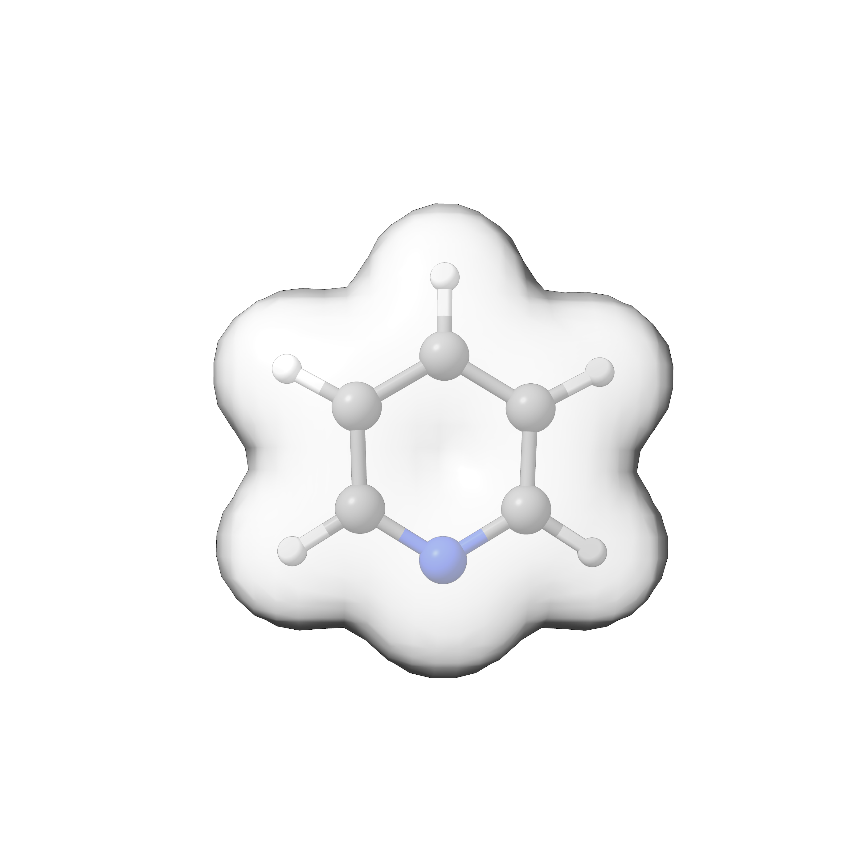
../../_images/orca_plot_pyridine_ElDens.png — Fig. 9.5 Pyridine SCF Electron Density¶

9.2.7.3. Perform Algebraic Operations¶

Starting from ORCA 6, one can perform simple algebraic operations with the computed densities. The presently available operations are listed in menu option 10:

Enter a number: 10
-----------------------------------------------------------------------
Available Algebraic Operations:
-----------------------------------------------------------------------
       1 - Pair Densities Addition
       2 - Pair Densities Subtraction
       3 - Pair Densities Multiplication
       4 - Pair Densities Division
       5 - Density Normalization
       6 - Make Natural Transition Orbitals
       7 - Make Natural Difference Orbitals
       8 - Leave Section - Return to Main Menu

To perform such operations, the desired state or transition-state densities must be available in the .densities file. This can be achieved by requesting the relevant densities to be written to disk using the !KeepDens or !KeepTransDensity keywords in the input.

NOTE: Storing hundreds or thousands of such densities requires care, as they may occupy hundreds of gigabytes of disk space.

In addition to the SCF calculation on pyridine, let us now perform a canonical CCSD calculation with the following input:

! CCSD def2-SVP KeepDens

*xyz 0 1
C        0.690940233      0.417992301     -1.170801378
C        0.690940233      1.616339301     -0.458357378
C        0.690940233      1.560238301      0.936438622
N        0.690940233      0.417992301      1.635468622
C        0.690940233     -0.724253699      0.936438622
C        0.690940233     -0.780354699     -0.458357378
H        0.690940233      0.417992301     -2.257043378
H        0.690940233      2.574997301     -0.967574378
H        0.690940233      2.478336301      1.521602622
H        0.690940233     -1.642351699      1.521602622
H        0.690940233     -1.739012699     -0.967574378
*       

Option 1 in the orca_plot menu will now provide both the scf and mdci electron densities.

-----------------------------------------------------------------------
Plot-Type is presently: 1
-----------------------------------------------------------------------
Searching for Ground State Electron or Spin Densities:              ...
-----------------------------------------------------------------------
     1 -   molecular orbitals                          
     2 -   (scf) electron density                              ......  (scfp                     )  => AVAILABLE
     3 -   (scf) spin density                                  ......  (scfr                     )  - NOT AVAILABLE
     4 -   natural orbitals                               
     5 -   corresponding orbitals                         
     6 -   atomic orbitals                                
     7 -   mdci electron density                               ......  (mdcip                    )  => AVAILABLE

Let us compute correlation electron density by taking the difference of CCSD and HF electron densities. Then, we need to choose option 2 (Pair Densities Subtraction) of the Available Algebraic Operations menu:

---------------------
List of density names
---------------------

Index:                                                   Name of Density
------------------------------------------------------------------------
    0:                                                pyridine_ccsd.scfp
    1:                                              pyridine_ccsd.P0.tmp
    2:                                               pyridine_ccsd.mdcip


-----------------------------------------------------------------------
Performing Algebraic Operations Over Densities: => SUBTRACTION
-----------------------------------------------------------------------
Number of Densities to be Processed from the List =>   2:
-----------------------------------------------------------------------
Enter FileName for Density[  0]: pyridine_ccsd.scfp
Provide a Scale Factor for Density[  0] (Default => 1.00): 1
Enter FileName for Density[  1]: pyridine_ccsd.mdcip
Provide a Scale Factor for Density[  1] (Default => 1.00): 1
-----------------------------------------------------------------------
INTERPRETTING EQUATION:
-----------------------------------------------------------------------
1/sqrt(N) * [(1.00) * {pyridine_ccsd.scfp} - (1.00) * {pyridine_ccsd.mdcip}]
-----------------------------------------------------------------------

PlotType       ... DENSITY-PLOT
ElDens File    ... pyridine_ccsd.scfp_minus_pyridine_ccsd.mdcip
Output file    ... pyridine_ccsd.scfp_minus_pyridine_ccsd.mdcip.cube
Format         ... Grid3d/Cube
Resolution     ... 80 80 80

The generated pyridine_ccsd.scfp_minus_pyridine_ccsd.mdcip.cube file can be directly visualized with a software like Chimera (see Fig. 9.6).

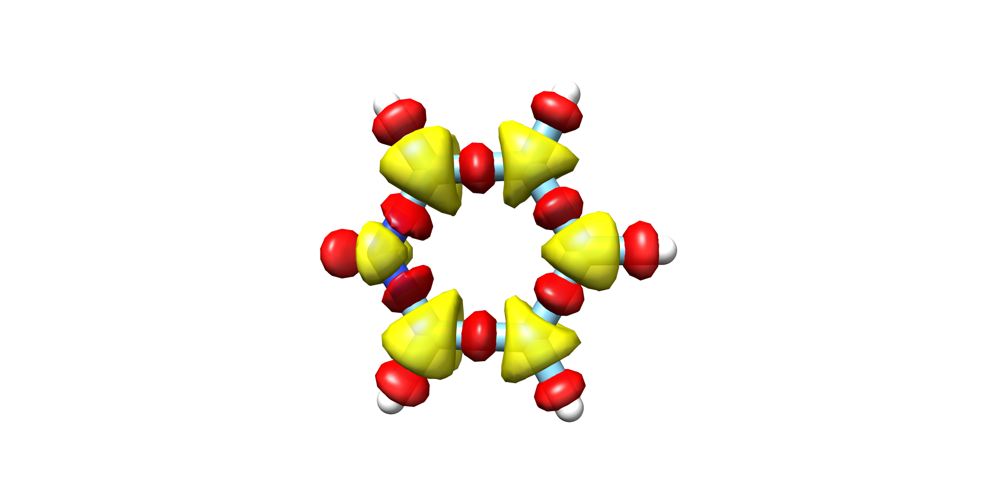
../../_images/orca_plot_pyridine_ElDens_CCSD_minus_HF.png — Fig. 9.6 Pyridine CCSD-HF Electron Density¶

NOTE: The generated density is stored in the Density Container so that it can be further processed or properly stored for future use. Now when option 9 is selected, the difference density will be seen among the available densities.

---------------------
List of density names
---------------------

Index:                                                   Name of Density
------------------------------------------------------------------------
    0:                                                pyridine_ccsd.scfp
    1:                                              pyridine_ccsd.P0.tmp
    2:                                               pyridine_ccsd.mdcip
    3:                      pyridine_ccsd.scfp_minus_pyridine_ccsd.mdcip

9.2.7.4. Plot Natural Transition Orbitals (NTOs) and Natural Difference Orbitals (NDOs)¶

orca_plot can also be used to generate Natural Transition Orbitals (NTOs) and Natural Difference Orbitals (NDOs) from any available state or transition density, regardless of the level of theory used. Let us now demonstrate this on the pyridine molecule for a state-averaged CASSCF(7,8) calculation. For this analysis, the relevant densities need to be stored to disk by including the !KeepTransDensity keyword in the input line. A corresponding ORCA input is as follows:

! def2-SVP KeepTransDensity 
  
%casscf
 nel 8
 norb 7
 mult 1
 nroots 10
end


*xyz 0 1
C        0.690940233      0.417992301     -1.170801378
C        0.690940233      1.616339301     -0.458357378
C        0.690940233      1.560238301      0.936438622
N        0.690940233      0.417992301      1.635468622
C        0.690940233     -0.724253699      0.936438622
C        0.690940233     -0.780354699     -0.458357378
H        0.690940233      0.417992301     -2.257043378
H        0.690940233      2.574997301     -0.967574378
H        0.690940233      2.478336301      1.521602622
H        0.690940233     -1.642351699      1.521602622
H        0.690940233     -1.739012699     -0.967574378
*

When this calculation is run, in addition to the CASSCF electron density, all relevant CASSCF state and transition densities become available, as can be seen by choosing option 1 in the main orca_plot menu:

-----------------------------------------------------------------------
Plot-Type is presently: 1
-----------------------------------------------------------------------
Searching for Ground State Electron or Spin Densities:              ...
-----------------------------------------------------------------------
     1 -   molecular orbitals                          
     2 -   (scf) electron density                              ......  (scfp                     )  => AVAILABLE
     3 -   (scf) spin density                                  ......  (scfr                     )  - NOT AVAILABLE
     ...
-----------------------------------------------------------------------
Searching for State or Transition State AO Electron Densities:      ...
-----------------------------------------------------------------------
    23 -   CIS unrelaxed transition AO density                 ......  (Tdens-CIS                )  - NOT AVAILABLE
    24 -   ROCIS unrelaxed transition AO density               ......  (Tdens-ROCIS              )  - NOT AVAILABLE
    25 -   CAS unrelaxed transition AO density                 ......  (Tdens-CAS                )  => AVAILABLE
    ...
-----------------------------------------------------------------------
Searching for State or Transition State MO Electron Densities:      ...
-----------------------------------------------------------------------
    29 -   CIS unrelaxed transition MO density                 ......  (Tdens-CISMO              )  - NOT AVAILABLE
    30 -   ROCIS unrelaxed transition MO density               ......  (Tdens-ROCISMO            )  - NOT AVAILABLE
    31 -   CAS unrelaxed transition MO density                 ......  (Tdens-CASMO              )  => AVAILABLE
   ...

We can now proceed to generate the NTOs and NDOs that dominate the computed State 1.

ROOT   1:  E=    -246.3609192216 Eh  5.176 eV  41749.8 cm**-1
      0.82391 [   346]: 2212100
      0.06447 [   295]: 2112200

With options 6 =>NTOs of the Available Algebraic Operations menu, one finds AO transition density \({D}_{01}\) file for NTOs as:

-----------------------------------------------------------------------
Performing Algebraic Operations Over Densities: => MAKE_NTOS
-----------------------------------------------------------------------
Enter FileName for Density[  0]: Tdens-CAS-0-0-0-1
Provide a Scale Factor for Density[  0] (Default => 1.00): 1
-----------------------------------------------------------------------
NATURAL TRANSITION ORBITALS GENERATION:
-----------------------------------------------------------------------
Warning: The one-electron matrix doesn't exist - is recalculated (SHARK)
Calculating the overlap matrix            ... done!

------------------------------------------------
NATURAL TRANSITION ORBITALS FOR STATE     1 1A  
------------------------------------------------

STATE    1 1A  :  E=   0.190226 au      5.176 eV    41749.8 cm**-1

Threshold for printing occupation numbers 1.0000e-04

     0  : n=  1.28519446
     1  : n=  0.03997952
     2  : n=  0.01505089
     3  : n=  0.00336119

=> Natural Transition Orbitals (donor   ) were saved in Tdens-CAS-0-0-0-1.1-1A_nto-donor.gbw
=> Natural Transition Orbitals (acceptor) were saved in Tdens-CAS-0-0-0-1.1-1A_nto-acceptor.gbw
-----------------------------------------------------------------------
Provide a Number of NTOs to plot (Default => 1): 1
-----------------------------------------------------------------------
-----------------------------------------------------------------------
Reading Donor NTO-file   : Tdens-CAS-0-0-0-1.1-1A_nto-donor.gbw
-----------------------------------------------------------------------
Generating cube file for Donor NTO[0]:=> Tdens-CAS-0-0-0-1.1-1A_nto-donor.gbw.0.cube
-----------------------------------------------------------------------
Reading Acceptor NTO-file   : Tdens-CAS-0-0-0-1.1-1A_nto-acceptor.gbw
-----------------------------------------------------------------------
Generating cube file for Acceptor NTO[0]:=> Tdens-CAS-0-0-0-1.1-1A_nto-acceptor.gbw.0.cube
Current-settings:

PlotType       ... MO-PLOT
MO/Operator    ... 0 0
Output file    ... Tdens-CAS-0-0-0-1.1-1A_nto-acceptor.gbw.0.cube
Format         ... Grid3d/Cube
Resolution     ... 80 80 80

With options 7 =>NDOs of the Available Algebraic Operations menu, one finds AO state density \(D_{00}-D_{11}\) file for NDOs as:

-----------------------------------------------------------------------
Performing Algebraic Operations Over Densities: => MAKE_NDOS
-----------------------------------------------------------------------
Enter FileName for Density[  0]: Tdens-CAS-0-0-0-0
Provide a Scale Factor for Density[  0] (Default => 1.00): 1
Enter FileName for Density[  1]: Tdens-CAS-0-0-1-1
Provide a Scale Factor for Density[  1] (Default => 1.00): 1
-----------------------------------------------------------------------
NATURAL DIFFERENCE ORBITALS GENERATION:
-----------------------------------------------------------------------
Warning: The one-electron matrix doesn't exist - is recalculated (SHARK)
Calculating the overlap matrix            ... done!

------------------------------------------------
NATURAL DIFFERENCE ORBITALS FOR STATE     1 1A  
------------------------------------------------

STATE    1 1A  :  E=   0.190226 au      5.176 eV    41749.8 cm**-1

Threshold for printing occupation numbers 1.0000e-04

     0  : n=  0.49881235
     1  : n=  0.08492368
     2  : n=  0.06708141
     3  : n=  0.01254920
     4  : n=  0.00667407
     5  : n=  0.00006162

=> Natural Difference Orbitals (donor   ) were saved in Tdens-CAS-0-0-0-0-Tdens-CAS-0-0-1-1.1-1A_ndo-donor.gbw
=> Natural Difference Orbitals (acceptor) were saved in Tdens-CAS-0-0-0-0-Tdens-CAS-0-0-1-1.1-1A_ndo-acceptor.gbw
-----------------------------------------------------------------------
Provide a Number of NDOs to plot (Default => 1): 1
-----------------------------------------------------------------------
-----------------------------------------------------------------------
Reading Donor NDO-file   : Tdens-CAS-0-0-0-0-Tdens-CAS-0-0-1-1.1-1A_ndo-donor.gbw
-----------------------------------------------------------------------
Generating cube file for Donor NDO[0]:=> Tdens-CAS-0-0-0-0-Tdens-CAS-0-0-1-1.1-1A_ndo-donor.gbw.0.cube
-----------------------------------------------------------------------
Reading Acceptor NDO-file   : Tdens-CAS-0-0-0-0-Tdens-CAS-0-0-1-1.1-1A_ndo-acceptor.gbw
-----------------------------------------------------------------------
Generating cube file for Acceptor NDO[0]:=> Tdens-CAS-0-0-0-0-Tdens-CAS-0-0-1-1.1-1A_ndo-acceptor.gbw.0.cube
Current-settings:

PlotType       ... MO-PLOT
MO/Operator    ... 0 0
Output file    ... Tdens-CAS-0-0-0-0-Tdens-CAS-0-0-1-1.1-1A_ndo-acceptor.gbw.0.cube
Format         ... Grid3d/Cube
Resolution     ... 80 80 80

Using the resulting cube file, one can readily visualize the corresponding Donor and Acceptor NTOs and NDOs orbital pairs as in which can be readily visualized in Fig. 9.7.

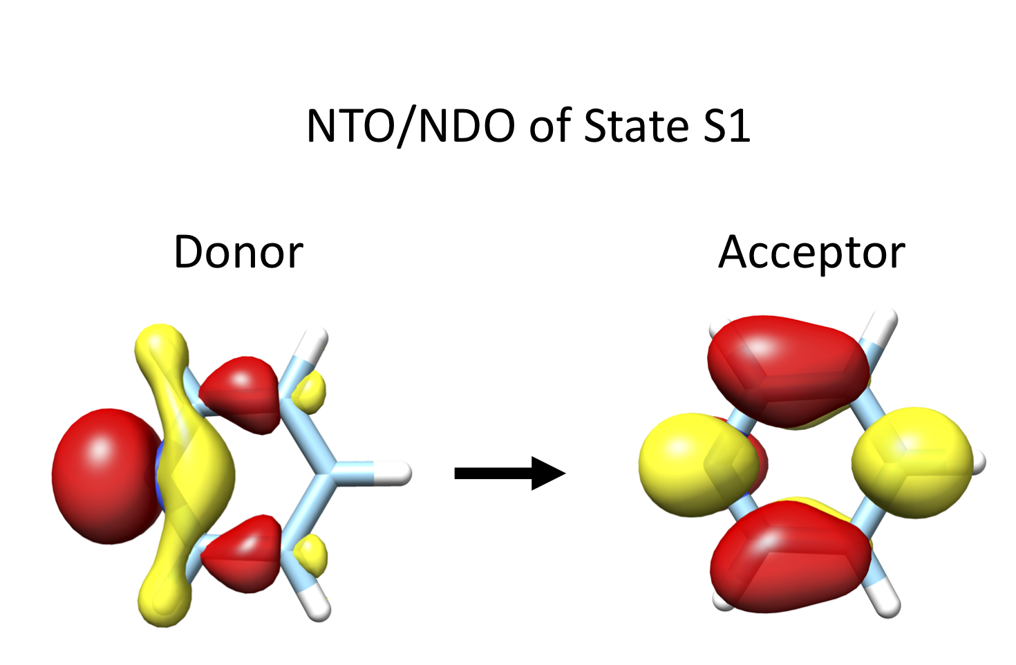
../../_images/orca_plot_pyridine_pyridine_s1_casscf_nto_ndo.png — Fig. 9.7 Pyridine SA-CASSCF(8,7) NTO/NDO donor/acceptor orbital pairs for State 1¶

NOTE: It is both beneficial and more accurate to always process AO-basis densities. In particular, it is neither possible nor correct to process reduced MO-basis densities.

9.2.7.5. Perform Electrostatic Potential Plots¶

Starting with ORCA 6.1, the electrostatic potential (ESP) can be generated in orca_plot for any state density available in the density container.

After performing an electronic structure calculation (e.g., using input), proceed as follows in orca_plot:

First, choose 1 - Enter type of plot, then select 43 - Electrostatic potential.

-   ROCIS QDPT unrelaxed transition AO density          ......  (Tdens-ROCISQDSOC         )  - NOT AVAILABLE
-   LFT QDPT unrelaxed transition AO density            ......  (Tdens-LFTQDSOC           )  - NOT AVAILABLE
-----------------------------------------------------------------------
-   Electrostatic Potential   

You will be prompted to specify the name of the state density for which the electrostatic potential is to be computed.

Enter Type: 43

---------------------
List of density names
---------------------

Index:                                                   Name of Density
------------------------------------------------------------------------
    0:                                                 pyridine_scf.scfp


Enter Name for an STATE Density: pyridine_scf.scfp

Finally, select option 11 - Generate the plot to compute the electrostatic potential and generate the file pyridine_scf.scfp.esp.cube.

The resulting .cube file contains the electrostatic potential data and may be visualized directly or used to color a density plot within any compatible graphical user interface tool.

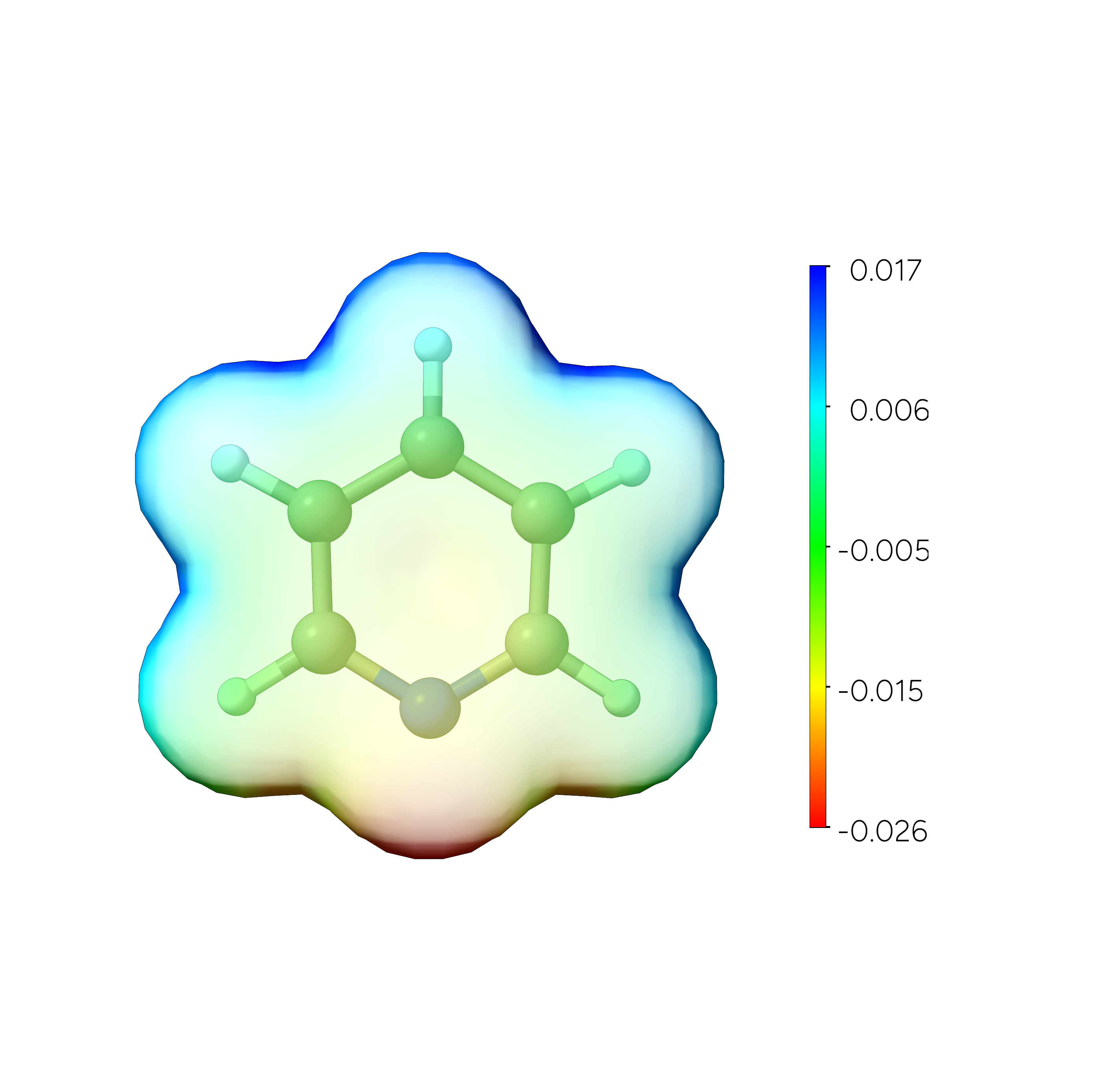
../../_images/orca_plot_pyridine_ElDens_ESPcolour.png — Fig. 9.8 Pyridine SCF Electron Density using ESP colouring¶

9.2.7.6. Additional TIPS regarding Density Plots¶

As an alternative to menu option 9, one can directly check which densities are available in the calculation directory by reading out the list of all densities contained in the .densities file:

orca_plot mymol.densities

orca_plot can also be run in parallel mode for computationally expensive plots:

mpirun -np 4 /orca_path/orca_plot_mpi MyGBWFile.gbw -i MyGBWFile

It is possible to use orca_plot to create difference densities between the ground and excited states from CIS or TD-DFT calculations directly from the .cis calculation information. This is implemented as an extra interactive menu point that is (hopefully) self-explanatory. Starting from ORCA 6 one can use the Algebraic Operations utility menu to carry out these operations directly from the generated State and Transition Densities.
It is also possible to use orca_plot to create difference densities between the ground and excited states from CIS or TD-DFT calculations using the .cis file. This functionality is implemented as an additional interactive menu option, which is (hopefully) self-explanatory. Starting from ORCA 6, these densities can also be obtained through the Algebraic Operations menu, processing directly the generated state and transition densities.

9.2.8. orca_2mkl: Old Molekel as well as Molden inputs¶

The orca_2mkl utility converts .gbw files into .mkl ASCII files. The .mkl file contains essentially the same information as the .gbw file, excluding ORCA-specific internal flags. The ASCII format makes it suitable for external use—for example, it can be read by Molekel for visualization or accessed by custom post-processing scripts. As such, .mkl files provide a convenient starting point for developing interfaces with third-party tools. orca_2mkl can be simply invoked as:

orca_2mkl BaseName 
      (will produce BaseName.mkl from BaseName.gbw)
orca_2mkl BaseName -molden
      (writes a file in molden format)
orca_2mkl BaseName -mkl
      (writes a file in MKL format)

Any gbw-like file, containing such as QRO, UNO, UCO, etc. orbitals, can be converted to the mkl and Molden formats using orca_2mkl:

orca_2mkl gbw_type_file.extension mkl_file.extension -mkl -anyorbs 
# or
orca_2mkl gbw_type_file.extension molden_file.extension -molden -anyorbs

orca_2mkl can also be run in reverse to generate .gbw type files from .mkl files:

orca_2mkl BaseName -gbw
      (will produce BaseName.gbw out of BaseName.mkl)

This functionality allows users to import molecular orbitals from external sources into ORCA. Although this feature is rarely used and offers limited capabilities, it is included here for users who wish to experiment. An example of this usage is demonstrated in the CASSCF tutorial accompanying the ORCA manual.

Finally, some third-party tools are available for converting the wavefunction files of other quantum chemistry programs from and to the MKL format, e.g. MOKIT (https://gitlab.com/jxzou/mokit). Combined with orca_2mkl, this provides a convenient way to use ORCA-generated molecular orbitals in other programs, or the other way around. One example application would be to use ORCA’s TRAH method to converge a difficult SCF problem, and pass the converged orbitals to another program that does not have the TRAH converger. Another example is to read in the orbitals of a difficult system from another program, and compute its high-level single point energy using ORCA using a functional or method that is not supported by the other program, without having to converge the wavefunction from the PModel guess. Finally, MOKIT can convert the MKL format to the PySCF format, which allows one to manipulate ORCA molecular orbitals in a Python environment.

9.2.9. orca_2aim¶

This utility program reads a .gbw file and creates a .wfn and .wfx file that can be used for topological analysis of the electron density by other programs. This works for open-shell and closed-shell wave functions. It can be invoked by including ! AIM in the simple input line of the ORCA input file, or typing in the terminal as follows:

orca_2aim BaseName 
      (will produce BaseName.wfn and BaseName.wfx from BaseName.gbw)

9.2.10. orca_vpot¶

This orca_vpot program calculates the electrostatic potential at a given set of user defined points. It can be used with either an input file or in interactive mode. It needs four arguments:

orca_vpot  MyJob.gbw  MyJob.scfp  MyJob.vpot.xyz  MyJob.vpot.out

First: The gbw file containing the correct geometry and basis set

Second: The desired density matrix in this basis (perhaps use the KeepDens keyword)

Third: an ASCII file with the target positions in AU, e.g.

               (number_of_points)
0 0.0  0.0    (XYZ coordinates)
 -5.0 0.0  0.0
0 5.0  0.0
0-5.0  0.0
0 0.0  5.0
0 0.0 -5.0

Fourth: The target file which will then contain the electrostatic potential, e.g.

6                 (number of points)
 VX1  VY1  VZ1    (potential for first point)
 VX2  VY2  VZ2    (potential for second point)
  etc.

It is straightforward to read this file and use the potential for intended purpose.

orca_vpot can be called in parallel mode as follows:

mpirun -np 4 /full_path/orca_vpot_mpi MyJob.gbw MyJob.scfp MyJob.pot.xyz MyJob.pot.out

It can be used to check available densities in MyJob.densities as:

orca_vpot  MyJob.densities

If the base names of the .gbw and .densities files do not match, the base name of the .densities file must be passed as the fifth argument:

orca_vpot  MyJob.gbw  OtherJob.scfp  MyJob.pot.xyz  MyJob.pot.out  OtherJob

A call to orca_vpot without any arguments will display a help message.

9.2.11. orca_euler¶

The orca_euler utility program calculates the relative orientation between calculated hyperfine coupling (HFC) or nuclear quadrupole coupling (NQC) tensors and a reference tensor,, typically the g-tensor or the D-tensor. The orca_euler program is invoked automatically at the end of an ORCA job if both the HFC/NQC and g-/D-tensor are calculated within the same run. Alternatively, it can be executed as a standalone program, provided that the .property.txt file from a previous NQC/HFC- and D- or g-tensor calculation is available.

The orientation between tensors is expressed as a 3×3 rotation matrix R, parameterized by the three Euler angles:\(\alpha\), \(\beta\) and \(\gamma\). These angles define the relative orientation of tensor A with respect to tensor B through three successive rotations around different axes to align A with B, i.e., in the commonly used z-y-z convention:

Rotate A\(_{xyz}\) counterclockwise around its \(z\) axis by \(\alpha\) to obtain A\(_{x'y'z'}\).
Rotate A\(_{x'y'z'}\) counterclockwise around its \(y'\) axis by \(\beta\) to obtain A\(_{x''y''z''}\).
Rotate A\(_{x''y''z''}\) counterclockwise around its \(z''\) axis by \(\gamma\) to align it with B.

The options of the orca_euler program are as follows:

orca_euler prop-file options

  file    = basename of an ORCA .property.txt file

  options  
   -refg/-refD:         Reference tensor (g-tensor or D-tensor, default is -refg)
   -conv zyz/-conv zxz: Euler rotation convention (default is zyz)
   -order:              Ordering of the reference tensor (x, y, z) with respect to 
                        ORCA output (min, mid, max)
   -plotA:              plot the HFC-tensors
   -plotQ:              plot the NQC-tensors
   -detail:             print detailed information

NOTE:

By default the D-tensor is used as reference tensor only if \(S\) >\(\frac{1}{2}\) and if D>0.3 cm\(^{-1}\). In all other cases, the g-tensor is used as reference tensor. The user can manually select the reference tensor (if available in the .property.txt file) by using –refg or –refD.
By default, the Euler rotation is performed using the z–y–z convention. The z-x-z convention can be selected manually by using the option –conv zxz.
By default, the axes of the g- or D-tensor are assigned based on the magnitude of their components: g\(_{\text{min} }\to g_{x}\), g\(_{\text{mid} }\to g_{y}\), g\(_{\text{max} }\to g_{z}\) (similarly for D). This ordering can be modified manually when running the standalone program, using the –order option as shown below:


-order 3 2 1:	min \(\to\) z
	mid \(\to\) y
	max \(\to\) x
-order 1 -2 3:	min \(\to\) x
	mid \(\to\) y (flipped in the orientation)
	max \(\to\) z

Files in .xyz format can be generated to plot nuclear hyperfine and quadrupole coupling tensors using the orca_euler program with the option –plotA or –plotQ. For example, the HFC tensor of atom 3 (counting starts at zero) is saved as prop-file.3.A.xyz, and the corresponding NQC tensor as prop-file.3.Q.xyz. These xyz files include four fictitious atoms (He, Ne, Ar, Kr), where the directions of the tensor axes are defined as vectors: x-axis from He to Ne; y-axis from He to Ar; and z-axis from He to Kr.
To print the actual definition of the rotation matrix and further information on the relative orientation, use the –detail option.

9.2.12. orca_exportbasis¶

The orca_exportbasis utility program prints out the basis sets used by ORCA. It requires the name of the basis set as specified in the ORCA input line. Optional arguments include an ECP basis set, a list of specific atoms, and the name of an output file. The output is written in ASCII format, which can be viewed and manually edited. Users can choose to export the basis sets in either ORCA format, which can be copied directlyinto the input file, or in GAMESS-US format, which can be used via the %basis block as externally specified basis.

NOTE: Basis set names containing special characters may require a pair of quotation marks (” or ‘) to be correctly recognized.

The usage and options of orca_exportbasis are as follows:

USAGE: orca_exportbasis keywords options

       -b, --basis  : name of basis set                                                        
                      def2-svp                                                                 
                      'def2-tzvp(-f)' - string to be passed with literals                       

EXAMPLE: orca_exportbasis -b svp

Additional Options:

       -e, --ecp    : ecp basis                                                                
                      sdd                                                                      
                      default        - ECP-part of basis (if present)                          

       -f, --format : output format                                                            
                      ORCA           - to be read via %basis NewGTO                           
                      GAMESS-US      - to be read as %basis GTOName 'mybasis.bas'             
                      default        - ORCA                                       
       -a, --atoms  : list of elements                                                         
                      Cu             - single element                                          
                      Ga Ge As Se    - list of elements separated by blanks                    
                      default        - whole periodic table is printed                         

       -o, --outfile: name of outputfile                                                       
                      mybasis.bas                                                              
                      default        - derived name                                            

EXAMPLE: orca_exportbasis -b svp -e sdd -a Ag -f GAMESS-US -o mybasis.bas

The output file stored in GAMESS-US format can be called in the %basis block of the next ORCA calculation - see Reading Basis Sets from a File.

%basis
GTOName      "mybasis.bas"
GTOAuxJName  "myauxjbasis.bas"
GTOAuxJKName "myauxjkbasis.bas"
GTOAuxCName  "myauxjcbasis.bas"
end

9.2.13. orca_eca¶

The orca_eca utility program uses the calculated exchange coupling constants to compute relative energies of all possible spin states by diagonalizing the spin Hamiltonian. The absolute and relative energies of the resulting spin states are printed in the *.en and *.en0 files, respectively. In addition, the on-site spin expectation values are written to a *.sp file. The following example calculates the spin ladder for a system with exchange coupling constant of -152.48 cm**-1 between Mn(III) and Mn(IV).

%sim
ms_bs 0.5 # Arbitrary spin state 
end

# specification of spin centers
$spins 2 
1 2.0  # Spin on first manganese
2 1.5  # Spin on second manganese

# Exchange coupling constant (H = -2J S1 S2)
$ecc 1
1 -152.48
    
$aiso_bs 2 # A false segment just to print the *.sp file
1 0.00
2 0.00

9.2.14. orca_pnmr¶

The orca_pnmr program calculates the paramagnetic contribution to the NMR shielding tensor using the EPR \(g\), \(A\), and \(D\) tensors (see Section Paramagnetic NMR Shielding Tensors for theoretical background). It is a standalone program that can be executed from the command line after the main ORCA calculation has finished. Alternatively, it can read user-provided \(g\)/\(A\)/\(D\) tensors from an input file using the option -i. Note that orca_pnmr expects \(g\) and \(A\) tensors to follow the conventions described in Section Cartesian Index Conventions for EPR and NMR Tensors.

The usage and options of orca_pnmr are as follows:

USAGE:    orca_pnmr BaseName [-i] [-v]

OPTIONS:  -i  : read from the input file "BaseName.pnmr.inp"
          -v  : print more output (Z matrices)

When run without any options, orca_pnmr attempts to extract the \(g\), \(D\), and \(A\) tensors from the file BaseName.property.txt and compute the paramagnetic shieldings at 298 K. This functionality only works if the tensors were computed using the EPRNMR module. A more flexible and controlled approach is to manually edit the BaseName.pnmr.inp (see below for its content) and then run orca_pnmr with the option –i.

3    # Spin multiplicity (2S+1)
298  # Temperature range minimum [K]
300  # Temperature range maximum [K]
1    # Temperature step [K]
1    # Have g-tensor? 0 or 1
  2.004689   0.000000  -0.000000 # Cartesian g-tensor
  0.000000   2.004689   0.000000 # (if available)
  0.000000   0.000000   2.002123
1    # Have D-tensor? 0 or 1
 -0.514341  -0.000000  -0.000000 # Cartesian D-tensor [cm-1]
 -0.000000  -0.514341  -0.000000 # (if available)
 -0.000000  -0.000000   1.028682
2    # Number of A-tensors
0O   # First nucleus (index,element)
-72.358765                       # Prefactor [MHz]
-78.989514   0.000000  -0.000000 # Cartesian A-tensor [MHz]
  0.000000 -78.989514  -0.000000
 -0.000000  -0.000000  53.478581
1O   # Next nucleus (index,element)
-72.358765                       # Prefactor [MHz]
-78.989516   0.000000  -0.000000 # Cartesian A-tensor [MHz]
  0.000000 -78.989516  -0.000000
 -0.000000  -0.000000  53.478580
# ... Further nuclei

The \(D\) and \(g\) tensors are optional. If they are not provided, orca_pnmr assumes an isotropic free-electron \(g\) value and sets \(D = 0\).
The \(A\) tensors are required. If no \(A\) tensor is provided for a given nucleus, the paramagnetic NMR shielding cannot be computed for that nucleus.

9.2.15. orca_lft¶

Starting from ORCA 5.0, ORCA features a standalone multiplet program called orca_lft.

orca_lft is dedicated to experimental spectroscopists.
It is able to run an arbitrary number of spectra simulations with emphasis on X-ray spectroscopies.

In this section we briefly review the main functionalities of orca_lft. For a more detail description and examples discussion, please refer to the orca_lft tutorial.

The goal is to be able to compute various spectroscopic properties of a given LFT center (ion) if one can manually pass the information of 1 and 2 electron integrals in the form of e.g the diagonal elements of the LFT matrix (LFT orbital energies) and the Slater-Condon parameters of a given LFT problem.
This will allow the experimental spectroscopist to perform a massive amount of spectra simulations during the actual running experiments

Any LFT problem can be parametrized in terms 1-electron \(H_{LF}\) matrix elements and the Slater-Condon 2-electron integrals F0, F2, F4, (or the Racah parameters A, B, C, of the d-shell). (Figure: Fig. 9.9)

../../_images/LFT_Integrals.svg — Fig. 9.9 Definition of an LFT problem in terms of 1-electron energies and Slater Condon parameters (SCPs)¶

In practice we need to know:

the Slater Condon parameters of a given LFT problem
the \(H_{LF}\) matrix elements or the relation of them (ligand field splitting, 10Dq, AOM model)

The design workflow of orca_lft is the following:

Solve the General CI problem on a User-specified LFT problem: Type of Ion, Number of Electrons, Involved Shells, Involved Multiplicities
Compute All possible Non Relativistic States/Multiplicity
Compute the Transition Densities on the CSFs basis
Compute the Needed transition Moments in the given LFT basis (i.e. 2p3d)
Compute various properties with emphasis to X-ray spectroscopy (ABS, XAS, XES, RIXS) at the Non Relativistic Limit
Compute the respective Relativistically corrected States on the Quasi Degenerate Perturbation Theory basis
Provide access to various relativistically corrected properies (ABS, XAS, XES, RIXS, MCD, XMCD, GTensors, Dtensors, Hyperfine Couplings, Electric Field Gradients)

orca_lft requires its own input. By simply executing it from the terminal

orca_lft

one gets printings for the usage:

************************************************************************************************************
Simulate or Fit Spectra
************************************************************************************************************

============================================================================================================
Usage: orca_lft BaseName.lft.inp [options]
============================================================================================================

------------------------------------------------------------------------------------------------------------
[Options]:
------------------------------------------------------------------------------------------------------------
-sim                          Simulate Spectra
-fit                          Fit Spectra (This is not yet availiable!)
------------------------------------------------------------------------------------------------------------

************************************************************************************************************
Generate Initial Input
************************************************************************************************************

============================================================================================================
Usage: orca_lft BaseName [options]
============================================================================================================

various Run Options:

------------------------------------------------------------------------------------------------------------
[Options]:
------------------------------------------------------------------------------------------------------------
-p_case                       Requests  p-shell case
-d_case                       Requests  d-shell case
-f_case                       Requests  f-shell case
-sp_case                      Requests sp-shell case
-ps_case                      Requests sp-shell case
-sd_case                      Requests sd-shell case
-ds_case                      Requests ds-shell case
-sf_case                      Requests sf-shell case
-fs_case                      Requests fs-shell case
-pd_case                      Requests pd-shell case
-dp_case                      Requests dp-shell case
-pf_case                      Requests pf-shell case
-fp_case                      Requests fp-shell case
-df_case                      Requests pf-shell case
-fd_case                      Requests fp-shell case
-spd_case                     Requests spd-shell case
-spf_case                     Requests spf-shell case
-sdf_case                     Requests sdf-shell case
-pdf_case                     Requests pdf-shell case
-soc                          Requests Input with SOC Constants
-atnoN                        Sets Atomic Number N
------------------------------------------------------------------------------------------------------------
-Special Cases for known Elements. LFT Parameters are filled from an internal AILFT NEVPT2 database

--------------------------------------Supported Oxidation States--------------------------------------------
Presently Default Oxidation States are supported except for Fe:
Main Elements                 -> O
TM Elements (Fe(26))          -> I,II,III
TM Elements (All other)       -> II
Lanthanide/Actinide Elements  -> III
--------------------------------------------Valence Cases---------------------------------------------------
-atnoN  -2s2p_case            Requests 2s2p-shell case for element with atomic number N (4-9)  
-atnoN  -3s3p_case            Requests 3s3p-shell case for element with atomic number N (12-18)
-atnoN  -4s4p_case            Requests 4s4p-shell case for element with atomic number N (20,31-36)
-atnoN  -4s4p_case            Requests 5s5p-shell case for element with atomic number N (38,49-54)
-atnoN  -3d4s_case            Requests 3d4s-shell case for element with atomic number N (22-29)
-atnoN  -4d5s_case            Requests 4d5s-shell case for element with atomic number N (40-47)
-atnoN  -5d6s_case            Requests 4d6s-shell case for element with atomic number N (72-79)
-atnoN  -4f5d_case            Requests 4d5d-shell case for element with atomic number N (59-70)
-atnoN  -5f6d_case            Requests 5d6d-shell case for element with atomic number N (91-102)
-----------------------------------------Core-Valence Cases------------------------------------------------
-atnoN  -1s3d_case            Requests 1s3d-shell case for element with atomic number N (22-29)
-atnoN  -2p3d_case            Requests 2p3d-shell case for element with atomic number N (22-29)
-atnoN  -3p3d_case            Requests 3p3d-shell case for element with atomic number N (22-29)
--------------------------------------Core-Valence XES Cases------------------------------------------------
-atnoN  -1s2p3d_case          Requests 1s2p3d-shell case for element with atomic number N (22-29)
-atnoN  -1s3p3d_case          Requests 1s3p3d-shell case for element with atomic number N (22-29)
------------------------------------------------------------------------------------------------------------

and various Spectra Simulation Options:

************************************************************************************************************
Spectra Simulation Options for the BaseName.lft.inp:
************************************************************************************************************

------------------------------------------------------------------------------------------------------------
TIP: Switch ON a Property calculation as DoProperty true:
------------------------------------------------------------------------------------------------------------

------------------------------------------------------------------------------------------------------------
General Input Parameters:
------------------------------------------------------------------------------------------------------------
NEl                           Sets the number of electrons
Shell_PQN                     Sets the principle quantum number per type of shells (s,p,d,f)
LFTCase                       !!!ALTERNATIVE TO Shell_PQN!!! Sets the given LFT problem (2p3d, 1s3p3d, ...)
----------------------------------------------------------------------------------------------------------- 
LFTCase WILL replace Shell_PQN                                                
----------------------------------------------------------------------------------------------------------- 
(e.g. Shell_PQN = 0,2,3,0 for a 2p3d calculation)
Mult                          Sets the Multiplicity/Multiplicities
NRoots                        Sets the number of Roots/Multiplicity
TMultiplets (0.01)            Threshold for the Multiplets grouping in eV
DoeV                          All values in eV. This is default. If set false the cm-1 unit is used throughout
DoRAS                         Requests a RASCI calculation
RAS(nel: m1 h/ m2 / m3 p)     Computes the X-Ray Emission Spectra

RAS-reference with nel electrons
m1= number orbitals in RAS-1
h = max. number of holes in RAS-1
m2= number of orbitals in RAS-2 (any number of electrons or holes)
m3= number of orbitals in RAS-3
p = max. number of particles in RAS-3

DoElastic                     Computes in addition the Elastic Scattering terms in RIXS/RIXSSOC calculations
------------------------------------------------------------------------------------------------------------
Non Relativistic Spectroscopic Properties:
------------------------------------------------------------------------------------------------------------
DoABS/DoXAS                   Computes the Absorption like Spectra
DoCD                          Computes the CD Spectra
DoXES                         Computes the X-Ray Emission Spectra
DoRIXS                        Computes the RIXS Spectra
DoQuadrupole                  Computes the ABS,XAS,RIXS Spectra beyond dipole approximation
------------------------------------------------------------------------------------------------------------
Relativistically Corrected Spectroscopic Properties:
------------------------------------------------------------------------------------------------------------
DoSOC                         Requests the Spin Orbit Coupling Calculations
Note that this turned on automatically if zeta SOC
constant are provided
------------------------------------------------------------------------------------------------------------
DoABS/DoXAS                   Computes the SOC Corrected Absorption like Spectra
DoCD                          Computes the SOC Corrected CD Spectra
DoMCD/DoXMCD                  Computes the SOC Corrected MCD/XMCD Spectra
DoXESSOC:                     Computes the SOC Corrected XES Spectra
DoRIXSSOC:                    Computes the SOC Corrected RIXS Spectra
DoQuadrupole                  Computes the SOC Corrected ABS,XAS, XES RIXS Spectra beyond dipole approximation
------------------------------------------------------------------------------------------------------------
Magnetic Properties:
------------------------------------------------------------------------------------------------------------
DoMagnetization               Computes the Magnetization
DoSusceptibility              Computes the Susceptibilities
DoGTensor                     Computes the g-Tensors/Matrices
DoDTensor                     Computes the Zero-Field Splittings
DoATensor                     Computes the Hyperfine Tensors
DoEFGTensor                   Computes the Electric Field Gradient Tensors
(also Moesbauer Parameters in the presence of Fe centers)
------------------------------------------------------------------------------------------------------------
Variable Parameters (if they are not given, default values are used)
------------------------------------------------------------------------------------------------------------
Temperature(300)              Temperature to be used in the SOC calculations
MagneticField(0)              Magnetic Field (in Gauss)
NPointsPsi(10)                Solid Angle Integration points Psi for MCD and XMCD
NPointsPhi(10)                Solid Angle Integration points Phi for MCD and XMCD
NPointsTheta(10)              Solid Angle Integration points Theta for MCD and XMCD
------------------------------------------------------------------------------------------------------------
Variable Parameters needed for Magnetization and Susceptibility calculations
------------------------------------------------------------------------------------------------------------
LebedevIntegrationPoints(26)  Number for Integration points for Lebedev)
LebedevPrec(5)                Precision of the grid for different field directions
(meaningful values range from 1 (smallest) to 10 (largest)
nPointsFStep (5)              Number of steps for numerical differentiation
(def: 5, meaningful values are 3, 5 7 and 9)
MAGTemperatureMIN(4.0)        Minimum Temperature (K) for Magnetization
MAGTemperatureMAX(4.0)        Maximum Temperature (K) for Magnetization
MAGTemperatureNPoints(1)      Number of Temperature points for Magnetization
MAGFieldStep(100.0)           Size of Field step for numerical differentiation (def: 100 Gauss)
MAGFieldMin(0.0)              Minimum Field (Gauss) for Magnetization
MAGFieldMax(70000.0)          Minimum Field (Gauss) for Magnetization
MAGNPoints(15)                Number of Field points for Magnetization
SUSTempMin(1)                 Minimum Temperature (K) for Susceptibility
SUSTempMxn(300.0)             Maximum Temperature (K) for Susceptibility
SUSNPoints(300)               Number of Temperature points for Susceptibility
SUSStatFieldMIN(0.0)          Minimum Static Field (Gauss) for Susceptibility
SUSStatFieldMAX(1)            Maximum Static field (Gauss) for Susceptibility
SUSStatFieldNPoints(1)        Number of Static Fields for Susceptibility
------------------------------------------------------------------------------------------------------------

orca_lft can run standalone by processing an input file (Basename.lft.inp) with orca_lft

orca_lft BaseName.lft.inp -sim

Alternatively, one can call the main orca program like

orca BaseName.lft.inp

The different benefits of the two runs are provided in the orca_lft tutorial

orca_lft can also be used to automatically generate initial proper input files. For example, an initial bare input file basename.lft_pd.inp can be generated by running

orca_lft BaseName -pd_case

-----------------------------------------------------------------
Initial Input: BaseName.lft_pd.inp for Orca_LFT has been generated: 
-----------------------------------------------------------------

The generated example input must be filled in with the required LFT parameters and the desired spectroscopic properties, after which the simulation can be started—just like in any standard multiplet program.

%lft


#-----Parameters------
NEl= 0
Shell_PQN= 0, 2, 3, 0
Mult= 0
NRoots= -1
#--------------------


#---Slater-Condon Parameters---
#---All Values in eV---
PARAMETERS
F0pp =  0.00
F2pp =  0.00
F0dd =  0.00
F2dd =  0.00
F4dd =  0.00
F0pd =  0.00
F2pd =  0.00
G1pd =  0.00
G3pd =  0.00
end
#--------------------


#---Diagonal LFT-Matrix Elelemnts---
#---All Values in eV---
FUNCTIONS
0   0 " 0.00"
1   1 " 0.00"
2   2 " 0.00"
3   3 " 0.00"
4   4 " 0.00"
5   5 " 0.00"
6   6 " 0.00"
7   7 " 0.00"
end
#--------------------


#---SPECTRA/PROPERTIES---
DoABS true
#---------
end


*xyz 0 0
Atom 0.00 0.00 0.00
*

Special initial inputs based on an internal NEVPT2 database can also be generated. For the 2p3d LFT case of Ni(II), this can be done as follows:

orca_lft BaseName -atno28 -2p3d_case

------------------------------------------------------------------------------
Creating input for Atom Ni(II) ...
------------------------------------------------------------------------------

-----------------------------------------------------------------
Initial Input: BaseName.lft_pd.inp for Orca_LFT has been generated: 
-----------------------------------------------------------------

The generated BaseName.lft_pd.inp file includes pre-filled LFT parameters from an internal NEVPT2 database, based on precomputed CASCI/NEVPT2 AILFT values. The resulting input-ready to runfor \(Ni^{II}\)-is as follows:

%lft


#-----Parameters------
NEl= 14
LFTCase 2p3d
Mult= 3, 1
NRoots= 25, 30
#--------------------


#---Slater-Condon Parameters---
#---All Values in eV---
PARAMETERS
F0pp =  85.88
F2pp =  54.77
F0dd =  23.31
F2dd =  13.89
F4dd =  9.14
F0pd =  33.03
F2pd =  7.76
G1pd =  6.42
G3pd =  2.11
end
#--------------------


#---Diagonal LFT-Matrix Elelemnts---
#---All Values in eV---
FUNCTIONS
0   0 " 0.00"
1   1 " 0.00"
2   2 " 0.00"
3   3 "1138.35"
4   4 "1138.35"
5   5 "1138.35"
6   6 "1138.35"
7   7 "1138.35"
end
#--------------------


#---SPECTRA/PROPERTIES---
DoABS true
#---------
end


*xyz 2 3
Ni 0.00 0.00 0.00
*

Alternatively, as discussed in the Ab initio Ligand Field Theory section (1- and 2-shell Abinitio Ligand Field Theory (AILFT)), one may actually run a 2-shell AILFT calculation and produce the respective .nevpt2.lft.inp file

!NoIter NEVPT2 def2-SVP def2-SVP/C


%method
frozencore fc_none
end

#--------------------
#Rotate Orbitals
#--------------------
%scf
rotate
{2,6,90}
{3,7,90}
{4,8,90}
end
end

#--------------------
#General Options
#--------------------
%casscf
nel 14
norb 8
mult 3,1
nroots 100,100

LFTCase 2p3d
rel
dosoc true
end
end


*xyz 2 3
Ni      0.0000000000      0.0000000000      0.0000000000
*

The structure of an orca_lft input is the following:

It contains:

The General Parameters Block where the LFT problem is defined

-----Parameters------ 
NEl= 14 
LFTCase 2p3d 
#Shells_PQN 0,2,3,0, Alternative definition using s,p,d,f main quantum numbers Mult= 3, 1
NRoots= 25, 30 
--------------------

The PARAMETERS Block where the SCPs and SOC constant parameters are defined

---Slater-Condon Parameters---
---All Values in eV--- 
PARAMETERS
F0pp = 85.88 
F2pp = 54.77 
F0dd = 23.31 
F2dd = 13.89 
F4dd = 9.14 
F0pd = 33.03 
F2pd = 7.76 
G1pd = 6.42 
G3pd = 2.11 
end 
--------------------

---SOC-CONSTANTS---
---All Values in eV--- 
PARAMETERS 
ZETA_P = 10.68
ZETA_D = 0.08 
end 
--------------------

The FUNCTIONS Block where the LFT matrix is defined

---Diagonal LFT-Matrix Elelemnts---
---All Values in eV--- 
FUNCTIONS
0   0 " 0.00"
1   1 " 0.00"
2   2 " 0.00"
3   3 "1138.35"
4   4 "1138.35"
5   5 "1138.35"
6   6 "1138.35"
7   7 "1138.35"
end
--------------------

The Properties Block where the desire simulation properties are specified
```
---SPECTRA/PROPERTIES--- 
DoABS true 
--------------------
```
The xyz Block where the ion, charge, multiplicity and coordinates (0. 0. 0.) are defined
```
*xyz 2 3 Ni 0.0000000000 0.0000000000 0.0000000000
```

Note

It should be emphasized the orca_lft through the FUNCTIONS and PARAMETERS subblocks provides

Arbitrary parameterization of both the one-electron LFT matrix and the Slater–Condon parameters
Powerful parameter scan capabilities

which helps to performs any kind of simulation without any symmetry restrictions. An example regarding the use of the FUNCTIONS and PARAMETERS subblocks is provided below, while a detailed orca_lft tutorial with worked out examples will be soon become available.

Let us perform the \(Ni^{2+}\) L-edge XAS spectrum simulation using the following input:

%lft


  #-----Parameters------
  NEl= 14
  LFTCase 2p3d
  Mult= 3, 1
  NRoots= 25, 30
  #--------------------
  
  
  #---Slater-Condon Parameters---
  #---All Values in eV---
  PARAMETERS
    F0pp =  85.88
    F2pp =  54.77
    F0dd =  23.31
    F2dd =  13.89
    F4dd =  9.14
    F0pd =  33.03
    F2pd =  7.76
    G1pd =  6.42
    G3pd =  2.11
  end
  #--------------------
  
  
  #---Diagonal LFT-Matrix Elelemnts---
  #---All Values in eV---
  FUNCTIONS
    0   0 " 0.00"
    1   1 " 0.00"
    2   2 " 0.00"
    3   3 "1138.35"
    4   4 "1138.35"
    5   5 "1138.35"
    6   6 "1138.35"
    7   7 "1138.35"
  end
  #--------------------
  
  #---SOC-CONSTANTS---
  #---All Values in eV---
  PARAMETERS
    ZETA_P = 11.341 
    ZETA_D = 0.085 
  end   
  #--------------------
  
  #---SPECTRA/PROPERTIES---
  DoABS true
  Rel
    DoSOC true
  End
  #---------
end


*xyz 2 3
Ni 0.00 0.00 0.00
*

Note

From ORCA 6.1 orca_lft is properly connected with the QDPT driver
This implies that all QDPT properties Magnetic Properties Through Quasi Degenerate Perturbation Theory can be requested within the Rel block

In the first step, the LFT problem at hand is defined:

------------------------------------------------------------------------------
                      L I G A N D    F I E L D    T H E O R Y
------------------------------------------------------------------------------


==============================================================================
                      LFT PARAMETERS DEFINITION BLOCK
==============================================================================


Number of electrons        = 14
Multiplicities             = 3 1 
Roots                      = 25 30 
Shells included            = 0 2 3 0 


----------------------------------------------------------
Definition of the ligand field basis set:
----------------------------------------------------------
   0  = pz     
   1  = px     
   2  = py     
   3  = dz2    
   4  = dxz    
   5  = dyz    
   6  = dx2y2  
   7  = dxy    


----------------------------------------------------------
Definition of the static ligand field by the user:
There are 11 ligand field parameters

----------------------------------------------------------
  Nr.               Name       Initial Value
  -----------------------------------------
    1               F0PP          85.880000
    2               F2PP          54.770000
    3               F0DD          23.310000
    4               F2DD          13.890000
    5               F4DD           9.140000
    6               F0PD          33.030000
    7               F2PD           7.760000
    8               G1PD           6.420000
    9               G3PD           2.110000
   10             ZETA_P          11.341000
   11             ZETA_D           0.085000


----------------------------------------------------------
Definition of the ligand field functions by the user:
There are 8 ligand field functions

----------------------------------------------------------
  Nr.      H-element         value   function
  ----------------------------------------------
 1   H(0,0)      0.000000000   0.00
 2   H(1,1)      0.000000000   0.00
 3   H(2,2)      0.000000000   0.00
 4   H(3,3)   1138.350000000  1138.35
 5   H(4,4)   1138.350000000  1138.35
 6   H(5,5)   1138.350000000  1138.35
 7   H(6,6)   1138.350000000  1138.35
 8   H(7,7)   1138.350000000  1138.35

After that, the CI problem is defined:

=> Defining the CI spaces and setting up the CI             ... 
==============================================================================
                             CI SETUP AND SOLUTION BLOCK
==============================================================================


Making Checks...
   Multiplicty =   3, #(configurations) =     28 #(CSF's) =     28 #(Roots) =     25 
   NRoots<NCSFs Adjussting  ==> (CSF's) =     25
Setting up CI...
   Multiplicty =   3, #(configurations) =     28 #(CSF's) =     25 #(Roots) =     25 
==============================================================================
                             CI SETUP AND SOLUTION BLOCK
==============================================================================


Making Checks...
   Multiplicty =   1, #(configurations) =     36 #(CSF's) =     36 #(Roots) =     30 
   NRoots<NCSFs Adjussting  ==> (CSF's) =     30
Setting up CI...
   Multiplicty =   1, #(configurations) =     36 #(CSF's) =     30 #(Roots) =     30 
CI setup done

Then, the CI problem is solved:

-----------------------------
 LFT-CI TRANSITION ENERGIES
------------------------------

LOWEST ROOT (ROOT 0, MULT 3) =    460.113216547 Eh 12520.317 eV

STATE ROOT MULT  DE/a.u.     DE/eV    DE/cm**-1
  1    3   0.000000     0.000      0.0
  2    3   0.000000     0.000      0.0
  3    3   0.000000     0.000      0.0
  5    3   0.000000     0.000      0.0
  4    3   0.000000     0.000      0.0
  6    3   0.000000     0.000      0.0
  0    1   0.086266     2.347  18933.2
  1    1   0.086266     2.347  18933.2
  2    1   0.086266     2.347  18933.2
  3    1   0.086266     2.347  18933.2
  4    1   0.086266     2.347  18933.2
  7    3   0.099001     2.694  21728.2
  8    3   0.099001     2.694  21728.2
  9    3   0.099001     2.694  21728.2
  5    1   0.132624     3.609  29107.7
  6    1   0.132624     3.609  29107.7
  7    1   0.132624     3.609  29107.7
  8    1   0.132624     3.609  29107.7
  9    1   0.132624     3.609  29107.7
 10    1   0.132624     3.609  29107.7
 12    1   0.132624     3.609  29107.7
 11    1   0.132624     3.609  29107.7
 13    1   0.132624     3.609  29107.7
 14    1   0.331652     9.025  72789.3
 15    1  29.897078   813.541 6561650.2
 16    1  29.897078   813.541 6561650.2
 17    1  29.897078   813.541 6561650.2
 18    1  29.897078   813.541 6561650.2
 19    1  29.897078   813.541 6561650.2
 10    3  29.915627   814.046 6565721.2
 11    3  29.915627   814.046 6565721.2
 13    3  29.915627   814.046 6565721.2
 12    3  29.915627   814.046 6565721.2
 14    3  29.915627   814.046 6565721.2
 15    3  29.915627   814.046 6565721.2
 16    3  29.915627   814.046 6565721.2
 17    3  29.978158   815.747 6579445.1
 18    3  29.978158   815.747 6579445.1
 19    3  29.978158   815.747 6579445.1
 20    3  29.978158   815.747 6579445.1
 21    3  29.978158   815.747 6579445.1
 22    3  30.016020   816.777 6587754.9
 23    3  30.016020   816.777 6587754.9
 24    3  30.016020   816.777 6587754.9
 20    1  30.087356   818.719 6603411.3
 21    1  30.087356   818.719 6603411.3
 22    1  30.087356   818.719 6603411.3
 23    1  30.106270   819.233 6607562.6
 24    1  30.106270   819.233 6607562.6
 25    1  30.106270   819.233 6607562.6
 26    1  30.106270   819.233 6607562.6
 27    1  30.106270   819.233 6607562.6
 29    1  30.106270   819.233 6607562.6
 28    1  30.106270   819.233 6607562.6

accompanied by a multiplet analysis:

---------------------------------------------------
Atomic calculation : Multiplet analysis (LFT)
---------------------------------------------------
multiplets found (Threshold = 0.01 eV)
3F | E =     0.000 eV | 2p(6)3d(8) 
3P | E =     2.694 eV | 2p(6)3d(8) 
3F | E =   814.046 eV | 2p(5)3d(9) 
3D | E =   815.747 eV | 2p(5)3d(9) 
3P | E =   816.777 eV | 2p(5)3d(9) 
1D | E =     2.347 eV | 2p(6)3d(8) 
1G | E =     3.609 eV | 2p(6)3d(8) 
1S | E =     9.025 eV | 2p(6)3d(8) 
1D | E =   813.541 eV | 2p(5)3d(9) 
1P | E =   818.719 eV | 2p(5)3d(9) 
1F | E =   819.233 eV | 2p(5)3d(9) 
---------------------------------------------------

This is followed by SOC computation in the QDPT framework:

*************************************
Doing QDPT with ONLY SOC!
*************************************

------------------------------------
NONZERO SOC MATRIX ELEMENTS (cm**-1)
------------------------------------

Bra                       Ket       
<Block Root  S    Ms  | HSOC |  Block Root  S    Ms>    =  Real-part     Imaginary part
--------------------------------------------------------------------------------------
0    1  1.0  1.0              0     0  1.0  1.0            0.000           -685.571
0    3  1.0  1.0              0     2  1.0  1.0            0.000            342.781
0    4  1.0  1.0              0     2  1.0  1.0            0.000              0.134
0    4  1.0  1.0              0     3  1.0  1.0            0.000             -2.946
0    5  1.0  1.0              0     2  1.0  1.0            0.000              0.987
0    5  1.0  1.0              0     3  1.0  1.0            0.000              7.920
0    5  1.0  1.0              0     4  1.0  1.0            0.000          -1022.995
0    6  1.0  1.0              0     2  1.0  1.0            0.000             -3.379

...

  1   29  0.0  0.0              0    17  1.0 -1.0        -2850.628           3039.103
1   29  0.0  0.0              0    18  1.0 -1.0        -16745.172           2885.219
1   29  0.0  0.0              0    19  1.0 -1.0        -1533.311           4672.283
1   29  0.0  0.0              0    20  1.0 -1.0          105.943            -43.140
1   29  0.0  0.0              0    21  1.0 -1.0           14.076             39.149

Note: In the following the full <I|HBO+SOC|J> are printed in the CI Basis.     
I,J are compound indices for |Block/Mult, Ms, Root>, where the states    
are ordered first by MultBlock, then Ms and finally Root.  

...

The corrected SOC states are then printed out:

The threshold for printing is 0.0010
Eigenvectors:
                         Weight      Real          Image    : Block Root    Spin   Ms
 STATE   0:       0.0000
                         0.014868    -0.121920     0.001813 :     0    0    1    1
                         0.158642     0.118778     0.380175 :     0    1    1    1
                         0.022316     0.003329     0.149347 :     0    2    1    1
                         0.073524    -0.037132     0.268598 :     0    3    1    1
                         0.071062    -0.251422     0.088592 :     0    4    1    1
                         0.068532    -0.250758     0.075180 :     0    5    1    1
                         0.010310     0.057750     0.083513 :     0    6    1    1
                         0.003333    -0.030103    -0.049264 :     0    0    1    0
                         0.007037     0.072029    -0.042999 :     0    1    1    0
                         0.245464     0.484256     0.104691 :     0    2    1    0
                         0.052920    -0.229815    -0.010229 :     0    3    1    0
                         0.017953     0.132002     0.022989 :     0    4    1    0
                         0.005423    -0.072174     0.014613 :     0    5    1    0
                         0.003723     0.024970     0.055669 :     0    6    1    0
                         0.018821     0.098122     0.095882 :     0    0    1   -1
                         0.081892    -0.206481     0.198135 :     0    1    1   -1
                         0.002458    -0.042784     0.025041 :     0    2    1   -1
                         0.057211    -0.099749     0.217397 :     0    3    1   -1
                         0.039565     0.098450     0.172838 :     0    4    1   -1
                         0.043388     0.182357     0.100666 :     0    5    1   -1
                         0.001044     0.019418     0.025827 :     0    6    1   -1
 STATE   1:       0.0000
                         0.042839    -0.206750    -0.009682 :     0    0    1    1
                         0.030129    -0.131357    -0.113467 :     0    1    1    1
                         0.004821    -0.067710    -0.015378 :     0    2    1    1
                         0.096567     0.259529     0.170915 :     0    3    1    1
                         0.019022    -0.134583    -0.030166 :     0    4    1    1
                         0.029125    -0.070877     0.155246 :     0    5    1    1
                         0.024443     0.150354     0.042856 :     0    6    1    1
                         0.126000    -0.140903    -0.325802 :     0    0    1    0
                         0.066620    -0.112104    -0.232493 :     0    1    1    0
                         0.034344    -0.075363    -0.169305 :     0    2    1    0
                         0.043496    -0.012839    -0.208161 :     0    3    1    0
                         0.035068    -0.017670     0.186428 :     0    4    1    0
                         0.088777    -0.019366    -0.297325 :     0    5    1    0
                         0.032394    -0.009435    -0.179735 :     0    6    1    0
                         0.033273    -0.179716    -0.031232 :     0    0    1   -1
                         0.038086    -0.175066     0.086245 :     0    1    1   -1
                         0.058972    -0.201976     0.134823 :     0    2    1   -1
                         0.091992     0.163866    -0.255226 :     0    3    1   -1
                         0.051908    -0.117870     0.194975 :     0    4    1   -1
                         0.015287    -0.106696    -0.062470 :     0    5    1   -1
                         0.036319     0.039383    -0.186462 :     0    6    1   -1
...
STATE 104: 6683223.2237
                         0.048335    -0.215907     0.041467 :     0   17    1    1
                         0.001350    -0.015566    -0.033287 :     0   18    1    1
                         0.058642    -0.018471    -0.241456 :     0   19    1    1
                         0.014743    -0.111453    -0.048181 :     0   20    1    1
                         0.019424    -0.128940     0.052904 :     0   21    1    1
                         0.013441    -0.042408    -0.107900 :     0   22    1    1
                         0.013136     0.106586    -0.042134 :     0   23    1    1
                         0.027360    -0.066625    -0.151399 :     0   24    1    1
                         0.030687     0.028711     0.172808 :     0   17    1    0
                         0.005134    -0.016659    -0.069691 :     0   18    1    0
                         0.006811    -0.016403    -0.080880 :     0   20    1    0
                         0.100510    -0.057415    -0.311791 :     0   21    1    0
                         0.054414    -0.044209    -0.229041 :     0   23    1    0
                         0.048345    -0.215766     0.042306 :     0   17    1   -1
                         0.001057    -0.001549     0.032472 :     0   18    1   -1
                         0.060316     0.071066     0.235085 :     0   19    1   -1
                         0.015880    -0.093356     0.084643 :     0   20    1   -1
                         0.019274    -0.138702    -0.005996 :     0   21    1   -1
                         0.013436    -0.004756     0.115817 :     0   22    1   -1
                         0.013139     0.114517     0.004987 :     0   23    1   -1
                         0.026471    -0.005403     0.162611 :     0   24    1   -1
                         0.050526     0.219718    -0.047434 :     1   20    0    0
                         0.293497    -0.532819     0.097985 :     1   21    0    0
                         0.064015     0.249661    -0.041039 :     1   22    0    0

Then, the SOC-corrected absorption (here XAS) spectrum is provided:

--------------------------------------------------------------------------------------------------------
      SOC CORRECTED ABSORPTION SPECTRUM VIA TRANSITION ELECTRIC DIPOLE MOMENTS    
--------------------------------------------------------------------------------------------------------
      Transition         Energy     Energy  Wavelength fosc(D2)      D2       |DX|      |DY|      |DZ|  
                          (eV)      (cm-1)    (nm)  (*population)  (au**2)    (au)      (au)      (au)  
--------------------------------------------------------------------------------------------------------
  1-3.0A  ->  2-3.0A    0.000000       0.0     0.0   0.000000000   0.00000   0.00000   0.00000   0.00000
  0-3.0A  ->  1-3.0A    0.000000       0.0     0.0   0.000000000   0.00000   0.00000   0.00000   0.00000
  0-3.0A  ->  2-3.0A    0.000000       0.0     0.0   0.000000000   0.00000   0.00000   0.00000   0.00000
  1-3.0A  ->  3-3.0A    0.000000       0.0     0.0   0.000000000   0.00000   0.00000   0.00000   0.00000
  2-3.0A  ->  3-3.0A    0.000000       0.0     0.0   0.000000000   0.00000   0.00000   0.00000   0.00000
  0-3.0A  ->  3-3.0A    0.000000       0.0     0.0   0.000000000   0.00000   0.00000   0.00000   0.00000
  1-3.0A  ->  4-3.0A    0.000000       0.0     0.0   0.000000000   0.00000   0.00000   0.00000   0.00000
  2-3.0A  ->  4-3.0A    0.000000       0.0     0.0   0.000000000   0.00000   0.00000   0.00000   0.00000
  2-3.0A  ->  5-3.0A    0.000000       0.0     0.0   0.000000000   0.00000   0.00000   0.00000   0.00000
  2-3.0A  ->  6-3.0A    0.000000       0.0     0.0   0.000000000   0.00000   0.00000   0.00000   0.00000
  0-3.0A  ->  4-3.0A    0.000000       0.0     0.0   0.000000000   0.00000   0.00000   0.00000   0.00000
  1-3.0A  ->  7-3.0A    0.000000       0.0     0.0   0.000000000   0.00000   0.00000   0.00000   0.00000
  1-3.0A  ->  6-3.0A    0.000000       0.0     0.0   0.000000000   0.00000   0.00000   0.00000   0.00000
  2-3.0A  ->  7-3.0A    0.000000       0.0     0.0   0.000000000   0.00000   0.00000   0.00000   0.00000
  1-3.0A  ->  5-3.0A    0.000000       0.0     0.0   0.000000000   0.00000   0.00000   0.00000   0.00000
  0-3.0A  ->  6-3.0A    0.000000       0.0     0.0   0.000000000   0.00000   0.00000   0.00000   0.00000
  0-3.0A  ->  7-3.0A    0.000000       0.0     0.0   0.000000000   0.00000   0.00000   0.00000   0.00000
  0-3.0A  ->  5-3.0A    0.000000       0.0     0.0   0.000000000   0.00000   0.00000   0.00000   0.00000
  1-3.0A  ->  8-3.0A    0.000000       0.0     0.0   0.000000000   0.00000   0.00000   0.00000   0.00000
  2-3.0A  ->  8-3.0A    0.000000       0.0     0.0   0.000000000   0.00000   0.00000   0.00000   0.00000
  0-3.0A  ->  8-3.0A    0.000000       0.0     0.0   0.000000000   0.00000   0.00000   0.00000   0.00000
  2-3.0A  ->  9-3.0A    0.171933    1386.7  7211.2   0.000000000   0.00000   0.00000   0.00000   0.00000
  1-3.0A  ->  9-3.0A    0.171933    1386.7  7211.2   0.000000000   0.00000   0.00000   0.00000   0.00000
  0-3.0A  ->  9-3.0A    0.171933    1386.7  7211.2   0.000000000   0.00000   0.00000   0.00000   0.00000
  1-3.0A  -> 10-3.0A    0.171933    1386.7  7211.2   0.000000000   0.00000   0.00000   0.00000   0.00000
  2-3.0A  -> 10-3.0A    0.171933    1386.7  7211.2   0.000000000   0.00000   0.00000   0.00000   0.00000
  0-3.0A  -> 10-3.0A    0.171933    1386.7  7211.2   0.000000000   0.00000   0.00000   0.00000   0.0

...

2-3.0A  -> 45-3.0A   808.419525 6520343.9     1.5   0.001132627   0.00052   0.01199   0.00520   0.01856
1-3.0A  -> 45-3.0A   808.419525 6520343.9     1.5   0.000466250   0.00021   0.00950   0.00818   0.00742
0-3.0A  -> 45-3.0A   808.419525 6520343.9     1.5   0.001659029   0.00075   0.01729   0.00696   0.02018
2-3.0A  -> 46-3.0A   808.419525 6520343.9     1.5   0.001163057   0.00053   0.01282   0.00222   0.01896
1-3.0A  -> 46-3.0A   808.419525 6520343.9     1.5   0.000718139   0.00033   0.00902   0.01359   0.00780
0-3.0A  -> 46-3.0A   808.419525 6520343.9     1.5   0.000710800   0.00032   0.01397   0.01112   0.00211
2-3.0A  -> 47-3.0A   808.419525 6520343.9     1.5   0.002893681   0.00132   0.02588   0.01640   0.01943
1-3.0A  -> 47-3.0A   808.419525 6520343.9     1.5   0.001285542   0.00058   0.02045   0.00869   0.00955
2-3.0A  -> 48-3.0A   808.419525 6520343.9     1.5   0.000921831   0.00042   0.00885   0.01380   0.01228

By processing the *.out file as usual with orca_mapspc orca_mapspc, the *.dat and *.stk files are generated. The XAS spectrum plotted using these files is given in Fig. 9.10.

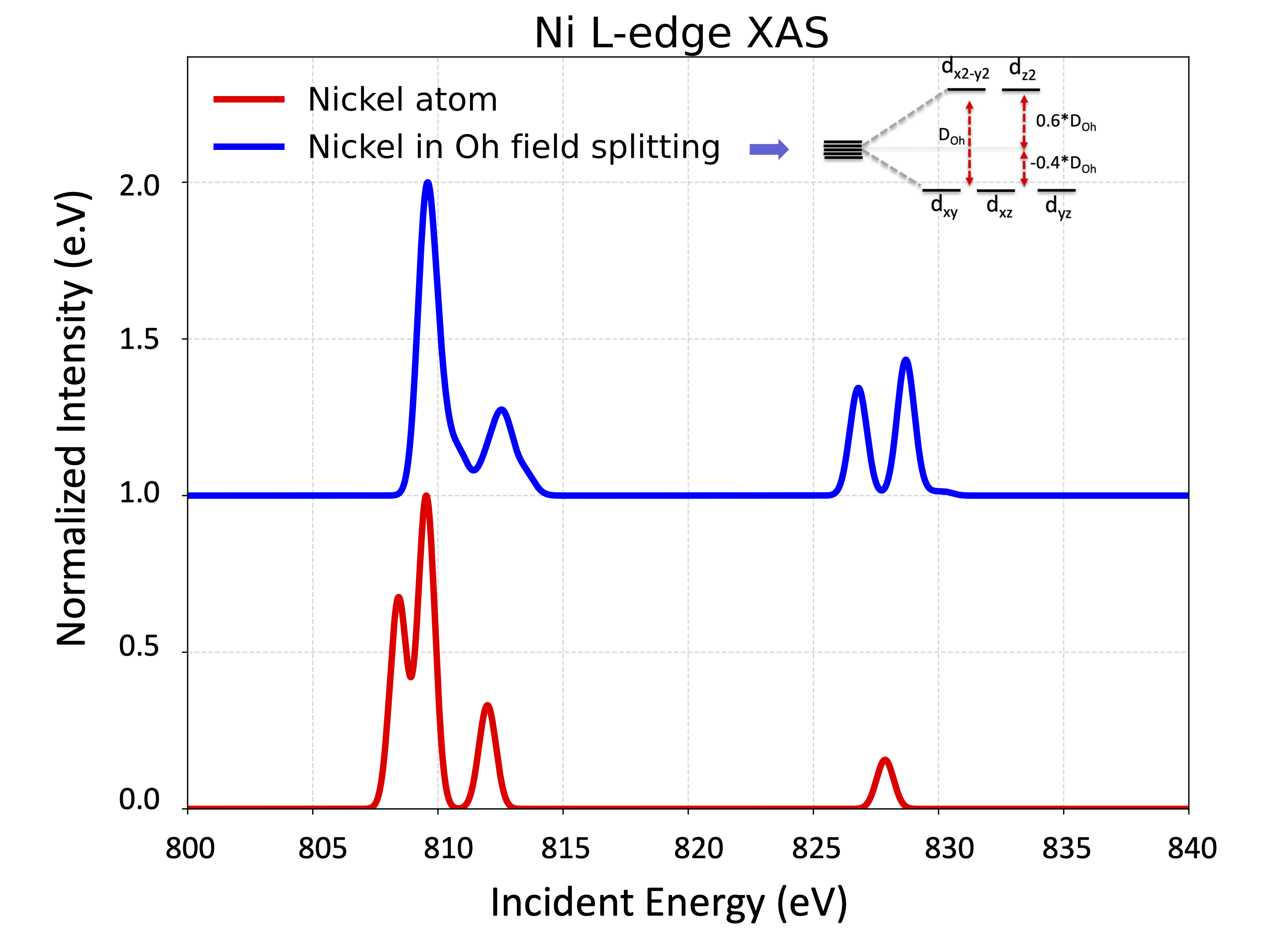
../../_images/Ni_L_edge_LFT_XAS.png — Fig. 9.10 orca_lft simulated \(Ni^{2+}\) L-edge XAS spectrum for the Nickel atom (red) and for the Nickel atom in the presence of an Oh field¶

The power of orca_lft stems from the fact that is entirely paramerizable. This flexibility is enabled through the intrinsic capabilities of the PARAMETERS and FUNCTIONS subblocks

Parameters Scanability Any given parameter—for example, the ZETA_D spin-orbit coupling (SOC) constant in the D-shell can be:
Switched on/off: ZETA_D= 0.0
Scanned over a range of parameters: ZETA_D= 0.0, 0.1, 11, which spans the range 0.0-0.1 eV for 11 steps.
Definition of New Parameters
Users may define any number or type of custom parameters within the PARAMETERS subblock: e.g. 10Dq= 1.2
Algebraic Relations in the PARAMETERS and FUNCTIONS Subblocks
Algebraic relations in the PARAMETERS subblock:

`DOh = 1.2`
`D1 = {-0.4*DOh}`
`D2 = {0.6*DOh}`

Algebraic relations in the FUNCTIONS subblock:

`3   3 "1138.35 + D2" # => dz2`
`4   4 "1138.35 + D1" # => dxz`

This provides the necessary flexibility to set up arbitrarily parameterized ligand field theory (LFT) models tailored to specific experimental chemical problems.

As an example, let us revisit the nickel complex discussed above and introduce a barycentric octahedral ligand field splitting of the d-orbital shell with 10Dq=1.2 eV.

The input now reads:

%lft


  #-----Parameters------
  NEl= 14
  LFTCase 2p3d
  Mult= 3, 1
  NRoots= 25, 30
  #--------------------


  #---Slater-Condon Parameters---
  #---All Values in eV---
  PARAMETERS
    F0pp =  85.88
    F2pp =  54.77
    F0dd =  23.31
    F2dd =  13.89
    F4dd =  9.14
    F0pd =  33.03
    F2pd =  7.76
    G1pd =  6.42
    G3pd =  2.11
    DOh = 1.2
    D1 = {-0.4*DOh}
    D2 = {0.6*DOh}
  end
  #--------------------


  #---Diagonal LFT-Matrix Elelemnts---
  #---All Values in eV---
  FUNCTIONS
    0   0 " 0.00"
    1   1 " 0.00"
    2   2 " 0.00"
    3   3 "1138.35 + D2" # => dz2
    4   4 "1138.35 + D1" # => dxz
    5   5 "1138.35 + D1" # => dyz
    6   6 "1138.35 + D2" # => dx2-y2
    7   7 "1138.35 + D1" # => dxy
  end
  #--------------------

  #---SOC-CONSTANTS---
  #---All Values in eV---
  PARAMETERS
    ZETA_P = 11.341
    ZETA_D = 0.085
  end
  #--------------------

  #---SPECTRA/PROPERTIES---
  DoABS true
  Rel
    DoSOC true
  End
  #---------
End

*xyz 2 3
Ni 0.00 0.00 0.00
*

By running the above inputone see that the new parameters DOH, D1 and D2 are succesfully defined:

----------------------------------------------------------
Definition of the ligand field basis set:
----------------------------------------------------------
= pz     
= px     
= py     
= dz2    
= dxz    
= dyz    
= dx2y2  
= dxy    


----------------------------------------------------------
Definition of the static ligand field by the user:
There are 14 ligand field parameters

----------------------------------------------------------
  Nr.               Name       Initial Value
  -----------------------------------------
             F0PP          85.880000
             F2PP          54.770000
             F0DD          23.310000
             F2DD          13.890000
             F4DD           9.140000
             F0PD          33.030000
             F2PD           7.760000
             G1PD           6.420000
             G3PD           2.110000
              DOH           1.200000
               D1          -0.480000
               D2           0.720000
           ZETA_P          11.341000
           ZETA_D           0.085000

And the Oh LFT splitting is take into account in the 1-electron LFT matrix as:

----------------------------------------------------------
Definition of the ligand field functions by the user:
There are 8 ligand field functions

----------------------------------------------------------
  Nr.      H-element         value   function
  ----------------------------------------------
 1   H(0,0)      0.000000000   0.00
 2   H(1,1)      0.000000000   0.00
 3   H(2,2)      0.000000000   0.00
 4   H(3,3)   1139.070000000  1138.35 + D2
 5   H(4,4)   1137.870000000  1138.35 + D1
 6   H(5,5)   1137.870000000  1138.35 + D1
 7   H(6,6)   1139.070000000  1138.35 + D2
 8   H(7,7)   1137.870000000  1138.35 + D1


=> Defining the one-electron LFT matrix                     ... done
----------------------------------------------------------
The ligand field one electron eigenfunctions:
----------------------------------------------------------
Orbital    Energy (eV) Energy(cm-1)          pz         px         py         dz2        dxz        dyz       dx2-y2       dxz
    1          0.000        0.0           1.000000   0.000000   0.000000   0.000000   0.000000   0.000000   0.000000   0.000000
    2          0.000        0.0           0.000000   1.000000   0.000000   0.000000   0.000000   0.000000   0.000000   0.000000
    3          0.000        0.0           0.000000   0.000000   1.000000   0.000000   0.000000   0.000000   0.000000   0.000000
    4       1137.870  9177541.4           0.000000   0.000000   0.000000   0.000000   1.000000   0.000000   0.000000   0.000000
    5       1137.870  9177541.4           0.000000   0.000000   0.000000   0.000000   0.000000   1.000000   0.000000   0.000000
    6       1137.870  9177541.4           0.000000   0.000000   0.000000   0.000000   0.000000   0.000000   0.000000   1.000000
    7       1139.070  9187220.1           0.000000   0.000000   0.000000   0.000000   0.000000   0.000000   1.000000   0.000000
    8       1139.070  9187220.1           0.000000   0.000000   0.000000   1.000000   0.000000   0.000000   0.000000   0.000000

Upon successful termination, one can process the Ni L-edge XAS spectrum and plot the resulting data, as shown in Fig. 9.10 (blue line), which indeed reproduces characteristic features of the Ni L-edge XAS spectrum of, for example, \(Ni(H_{2}O)_6\).

Note

A detailed tutorial will soon become available that further explores the capabilites of orca_lft

9.2.16. orca_crystalprep¶

ORCA features a utility program orca_crystalprep that can process crystallographic .cif files or .xyz supercell files and produce proper inputs for the embedded cluster calculations.

To perform an embedded cluster calculation conventionally or within the Ionic-Crystal-QMMM, one needs to define basically 3 regions:

The quantum cluster QC that will be treated quantum mechanically.
The point charge region PC that represents the solid’s environment.
A boundary region BR or ECP that is located between the QC and PC with the main role to prevent charge communication between the QC and PC regions.

This implies that, in the first step, a SuperCell (.xyz) must be generated, with different regions separated according to the calculation design. In the second step, the charge of the system must be balanced. Finally, all these need to be combined into a proper calculation input.

This is clearly a multistep and many times multiplatform process that is

complicated,
time consuming,
not user friendly.

The orca_crystalprep utility is designed to automatically generate proper inputs for ORCA embedded cluster calculations with the aim to allow to a wide range of experienced and not experienced users the ability to setup an embedded cluster calculation with a minimal effort.

orca_crystalprep requires its own input. By simply executing it from the terminal:

orca_crystalprep

one gets printings for the usage

************************************************************************************************************
Generate initial ORCA CrystalPrep Input
************************************************************************************************************

============================================================================================================
Usage: orca_crystalprep [Basename Input] [options]
============================================================================================================

------------------------------------------------------------------------------------------------------------
[Options]:
------------------------------------------------------------------------------------------------------------
-geninput                     Generate Initial Input
------------------------------------------------------------------------------------------------------------

************************************************************************************************************
Generate ORCA Embedding Cluster Inputs using the CrystalPrep Utility
************************************************************************************************************

============================================================================================================
Usage: orca_crystalprep [CrystalPrep Input]
============================================================================================================

and the different options:

------------------------------------------------------------------------------------------------------------
[CrystalPrep Input Options]:
-------------------------------------------------------------------------------------------------------------
General Definitions
-------------------------------------------------------------------------------------------------------------
DoCIF                       true                     This will process a .cif file                         
DoXYZ                       true                     This will process a .xyz file                         
InputCIF                    "CIFFileName"            Set the name of the CIFFileName                     
InputXYZ                    "XYZFileName"            Set the name of the XYZFileName                     
-------------------------------------------------------------------------------------------------------------
SuperCell Construction Definitions
-------------------------------------------------------------------------------------------------------------
DoSuperCell                 true                     Flag to generate a SuperCell                          
SCDimension                 "axbxc"                  The Dimension of the SuperCell (e.g. "1x1x1")     
InputCIF                    "CIFFileName"            Set the name of the CIFFileName                     
InputXYZ                    "XYZFileName"            Set the name of the XYZFileName                     
-------------------------------------------------------------------------------------------------------------
Special Tasks on SuperCells
-------------------------------------------------------------------------------------------------------------
DoFractional                 true                    Flag to Transform Cartesian to Fractional coordinates   
DoSymmetryOperations         true                    Flag to enforce using built in Symmetry Operations      
DoHemiSphereSC               true                    Flag to request a Hemisphere Super Cell build           
DoSymetricSC                 true/false              Flag to request a Symmetric Super Cell build            
                             false => Origin Build    :  0 - ra,   0 - rb,   0 - rc  => Default for Now!                     
                             true  => Symmetric Build :  -ra - ra, -rb - rb, -rc - rc                                         
-------------------------------------------------------------------------------------------------------------
Embedding Cluster Definitions
-------------------------------------------------------------------------------------------------------------
DoEmbedding                  true                    Flag to generate the files for the embedding approach   
UseVolumeCriterion           true                    Volume Criterion to generate layers                     
UseDistanceCriterion         true                    Distance Criterion to generate layers                   
CellVolumeFraction           value                   Cell(UniCell/SuperCell) fraction (default 1.0)          
DoMolecularFragments         value                   Define Molecular Fragments during the build             
DoSimpleInput                true                    Flag to generate a conventional Embedding Cluster input 
DoICQMMMInput                true                    Flag to generate a Ionic-Crystal-QMMM input             
DoMCQMMMInput                true                    Flag to generate a Mol-Crystal-QMMM input               
WritePDB                     true                    Flag to run a Ionic-Crystal-QMMM input from a PDF file  
QCCharge                     Charge Number           Specify the total QC Charge                             
QCMult                       Multiplicity Number     Specify the total Multiplicity                          
-------------------------------------------------------------------------------------------------------------
Special Tasks on Embedding Cluster Construction/Definition
-------------------------------------------------------------------------------------------------------------
DoLayers                     true                    Request Layers Definition                               
1) Layers Definition. There are 2 Options:                                                                   
             a) The Differnt regions are build in layers as multipoles of the UnitCell                       
             b) The Differnt regions are build in layers around a predefined QC cluster via a QCAtom List    
QCLayers                     QC Layers Number        Specify the number of the QC Layers                     
ECPLayers                    ECP Layers Number       Specify the number of the ECP Layers                     
PCLayers                     PC Layers Number        Specify the number of the PC Layers                     
HFLayers                     HF Layers Number        Specify the number of the HF Layers                     
Example Input
QCLayers 1 
2) Atoms Definition. This is alternative to Layers Definition (e.g. DoLayers false)                          
NQCAtoms                     QC Atoms  Number        Specify the number of the QC Atoms                      
NHFAtoms                     HF Atoms  Number        Specify the number of the HF Atoms                      
NECPAtoms                    ECP Atoms  Number       Specify the number of the ECP Atoms                     
NPCAtoms                     PC Atoms  Number        Specify the number of the PC Atoms                      
QCAtoms                      QC Atoms  List          Specify the List   of the QC Atoms (e.g. 0,1,4,10...    
HFAtoms                      HF Atoms  List          Specify the List   of the HF Atoms (e.g. 0,1,4,10...    
ECPAtoms                     ECP Atoms  List         Specify the List   of the ECP Atoms (e.g. 0,1,4,10...   
PCAtoms                      PC Atoms  List          Specify the List   of the PC Atoms (e.g. 0,1,4,10...    
Example Input
NQAtoms= 4 
QCAtoms 0,1,4,10 
-------------------------------------------------------------------------------------------------------------
Request an Explicit Atom Definion in Ionic-Crystal-QMMM 
HINT: This is automatically Set to true if an Atom List (QC Atoms, ECP Atoms, ...) is provided by the user
-------------------------------------------------------------------------------------------------------------
SetQCAtoms                   true                    Set explicitely the QC Atoms                            
SetHFAtoms                   true                    Set explicitely the HF Atoms                            
SetECPAtoms                  true                    Set explicitely the ECP Atoms                           
SetPCAtoms                   true                    Set explicitely the PC Atoms                            
SetPC2Atoms                  true                    Set explicitely the PC2 Atoms                           
-------------------------------------------------------------------------------------------------------------
Load a User Defined QC Cluster
-------------------------------------------------------------------------------------------------------------
LoadQCCluster                true                    Load the QC Cluster                                     
InputXYZ                   "QCXYZFileName"         Set the name of the QC XYZFileName                      
-------------------------------------------------------------------------------------------------------------
NOTE: This ALWAYS requires to build symmetric Super Cells. Hence DoSymetricSC turns on by default!           
-------------------------------------------------------------------------------------------------------------
STEPS:                                                                                                       
      1) Build a minimal (1x1x1 or 2x2x2) and define the QC cluster that is saved as QCXYZFileName           
      2) Build the actual SuperCell (e.g. 10x10x10) by Loading the QC cluster                                
         and define the QC cluster that is saved as QCXYZFileName                                            
      3) Build the Embedded Cluster around the Loaded QC employin the Layers scheme                          
-------------------------------------------------------------------------------------------------------------
Redefine SuperCell Origin. This is for shifting the center origin to a desired atom during the SC Construction  
This Helps to automatically construct desired Cluster structures using the Layers Definition 
-------------------------------------------------------------------------------------------------------------
ShiftOrigin                  true                    Request Origin Shift  to a particular Atom              
ChosenAtom                   an Atom Number          The Number of the Chosen atom (e.g. 2)                  
-------------------------------------------------------------------------------------------------------------
Neutralize the Embedded Cluster in the Simple Input
Note that in the Ionic-Crustal QMMM Input this step is taken care on demand during the QM/MM run
-------------------------------------------------------------------------------------------------------------
ChargePoints                the charge points        Specify the number of the charge points (default 1000)  
ChargeStep                  the charge points        Define the step during the iterations (default 0.01)    
ChargeThres                 the threshold            Define the neutralization threshold (default 0.01)      
Neutralization Schemes:                                                                                      
NeutralizingScheme1         true                 ->  Neutralization is based on All Charges                  
NeutralizingScheme2         true                 ->  Neutralization is based on different charges            
                                                     Equiping the ECP and PC regions                         
NeutralizingScheme3         true                 ->  Neutralization is based on PC2 Region                   
-------------------------------------------------------------------------------------------------------------
Special Definitions for the .metainfo File in the Ionic-Crustal QMMM
This helps Setting Charge/Spin in a specific atom type
It can also aid the neutralization step of the Embedded Cluster in the Simple Input 
-------------------------------------------------------------------------------------------------------------
NAtomTypes                  Number of Atom Types     Specify The Atom types that will be defined             
Example Input
#-------------------------
#Atom Type Charge Spin
#-------------------------
AtomTypes 2
Co    1    2.0   1.5
Co    2    3.0   0
end
This specifies the local Spin and Charge of a Td HS Co2+ center (Type 1) and a OH Co3+ center (Type 2)
During the Embedding cluster construction
-------------------------------------------------------------------------------------------------------------

In the first step, the orca_crystalprep tool can be used to generate its own input by running:

orca_crystalprep crystalprep.inp -geninput

This will generate an initial input:

---------------------------------------------------------------------------------
Initial Input: crystalprep.inp for Orca_CrystalPrep has been generated. All Done! 
---------------------------------------------------------------------------------

It looks like the following:

%crystalprep


#************************
#Read CIF/XYZ
#************************
DoCIF true  

#------------------------
#INPUT CIF/XYZ
#------------------------
#InputCIF "CIFName.cif"
#------------------------
#Set Special Tasks
#------------------------
#SpaceGroupNumber 200

#************************
#Generate SuperCell      
#************************
DoSuperCell true
SCDimension "1x1x1"

#************************
#Setup Embedding Approach
#************************
DoEmbedding true
DoLayers true

#------------------------
#Atom Type Charge Spin
#------------------------
#NAtomTypes 2
#Co 1 2.0  1.5
#Co 2 3.0  0.0

#************************
#Generate Inputs
#************************
#DoSimpleInput true
#DoICQMMMInput true

#Neutralize true
#QCCharge 0
#QCMult 1
#------------------------
end

As outlined in Fig. 9.11, by specifying the names of the desired *.cif or *.xyz file along with the appropriate options, a ready-to-run embedding cluster input can be generated.

../../_images/CrystalPrep_ICQMMM.svg — Fig. 9.11 Embedded cluster IC-QM/MM Input generation¶

By default, the embedded cluster structure is constructed using a layer-based approach, in which different structural layers are generated as multiples—or fractions—of the unit cell.

The unit cell fractions, expressed in terms of volume units, are specified using the following keyword:

CellVolumeFraction N #by default N=1

As an example, let us consider the NaCl case in detail . We aim to generate a complete embedding cluster setup that includes:

a 20x20x20 supercell, constructed from the nacl.cif file,
an embedding cluster with 1 QC layer and 1 ECP layer, and
an IC-QM/MM embedding cluster input

These can be prepared with the following ORCA input file calling orca_crystalprep program through the %crystalprep block:

%crystalprep


#************************
#Read CIF/XYZ
#************************
DoCIF true

#------------------------
#INPUT CIF/XYZ
#------------------------
InputCIF "nacl.cif"

#************************
#Generate SuperCell
#************************
DoSuperCell true
SCDimension "20x20x20"

#************************
#Setup Embedding Approach
#************************
DoEmbedding true
DoLayers true

#------------------------
#Atom Type Charge Spin
#------------------------
NAtomTypes 2
Na 0  1.0  0.0
Cl 1 -1.0  0.0

#************************
#Generate Inputs
#************************
DoICQMMMInput true
QCCharge 0
QCMult 1  
#------------------------
end

In the first step, the orca_crystalprep processes the nacl.cif file and creates the unit cell and the requested 20x20x20 supercell:

-------------------------------------------------------------
Reading Information from the provided CIF file: nacl.cif
-------------------------------------------------------------

------------------------Unit Cell Parameters-----------------
Hermann-Mauguin Space Group:     P1
Space Group ID:                1
Unit Cell Symmetry:                
Unit Cell Volume:             46.09
Unit Cell alpha angle:        60.00
Unit Cell beta angle:         60.00
Unit Cell gamma angle:        60.00
Unit Cell alpha length:       4.024
Unit Cell beta length:        4.024
Unit Cell gamma length:       4.024
Atom   Type   AO    x     y     z    occ
Na     0     11 0.000 0.000 0.000  1.00
Cl     1     17 0.500 0.500 0.500  1.00
Done
-------------------------------------------------------------

----------Making a SuperCell with 20x20x20 dimensions-----------
Unit Cell:
0          1          2    
0       4.024000   0.000000   0.000000
1       0.000000   4.024000   0.000000
2       0.000000   0.000000   4.024000

Transformation Matrix:
0          1          2    
0      80.480000   0.000000   0.000000
1       0.000000  80.480000   0.000000
2       0.000000   0.000000  80.480000


---------------------------------------------------------------------
Saving xyz file: nacl4.cif_20x20x20.xyz                   ...Done
---------------------------------------------------------------------

Then, the costruction of the embedding cluster structure is initiated:

------------Making a Embedding Cluster Input ------------
------------Using the Layers Approach with: ------------
QC_Layers: 1
ECP_Layers: 1
PC_Layers: 1
--------------
Preparing Inputs ...

In the next step, the center of the supercell (.xyz) is assigned to the closest atom to the center:

-------------------------------
The Center of XYZ Coordinates
-------------------------------
41.246, 41.246, 41.246
-------------------------------
Closest Atom to Center
-------------------------------
Na(4630) 40.240, 40.240, 40.240
-------------------------------
Shifting Origin to closest atom
-------------------------------
40.240, 40.240, 40.240

After that, layers are generated automatically:

--------------------------------------
Saving Generated Layers XYZ Files ...
--------------------------------------
Saving Layer 0 XYZ File: nacl.cif_20x20x20.xyz_0.xyz
Saving Layer 1 XYZ File: nacl.cif_20x20x20.xyz_1.xyz
Saving Layer 2 XYZ File: nacl.cif_20x20x20.xyz_2.xyz
Saving Layer 3 XYZ File: nacl.cif_20x20x20.xyz_3.xyz
Saving Layer 4 XYZ File: nacl.cif_20x20x20.xyz_4.xyz
Saving Layer 5 XYZ File: nacl.cif_20x20x20.xyz_5.xyz
Saving Layer 6 XYZ File: nacl.cif_20x20x20.xyz_6.xyz
Saving Layer 7 XYZ File: nacl.cif_20x20x20.xyz_7.xyz
Saving Layer 8 XYZ File: nacl.cif_20x20x20.xyz_8.xyz
Saving Layer 9 XYZ File: nacl.cif_20x20x20.xyz_9.xyz

--------------------------------------
Saving Generated Layers PDB File ...
--------------------------------------

This is followed by the embedding cluster construction:

--------------------------------------
Saving Generated Cluster XYZ Files ...
--------------------------------------
Saving QC XYZ File: nacl.cif_20x20x20.xyz_QC.xyz
Saving ECP Region XYZ File: nacl.cif_20x20x20.xyz_ECP.xyz
Saving PC Region XYZ File: nacl.cif_20x20x20.xyz_PC.xyz

Finally, the IC-QM/MM embedding cluster is generated:

--------------------------------------
Saving Embedding Cluster Inputs ...
--------------------------------------
Saving ICQMMM Input: nacl.cif_20x20x20.xyz.ICQMMM.inp
Done
--------------------------------------------------------------

Ionic-Crystal QM/MM calculations require the generation of a simple force field, which is stored in a *.prms file, as described in section Overview on ORCA’s Multiscale Implementation. The necessary information, including charge and spin, is taken from a .metainfo file. The orca_crystalprep tool allows for externally setting the charge and spin in the .metainfo file, as described below:

First, during processing of the .cif file, atom types are assigned to all atoms detected in the asymmetric unit.

Atom   Type   AO    x     y     z    occ
Na     0     11 0.000 0.000 0.000  1.00
Cl     1     17 0.500 0.500 0.500  1.00

In the orca_crystalprep input, the charge and spin of specific atom types can be assigned as follows:

NAtomTypes 2
Na 0  1.0  0.0
Cl 1 -1.0  0.0

This information is then passed in the .metainfo file


# atom nr. - element - atom type - formal charge - formal spin - molecule nr
Na   0  1  0           1
Na   0  1  0           1
Na   0  1  0           1
...

Cl   1 -1  0        1
Cl   1 -1  0        1
Cl   1 -1  0        1
...

After completing the preparatory steps, the embedded cluster is constructed as shown in Fig. 9.12.

../../_images/Embedded_Cluster.svg — Fig. 9.12 Generated Embedded cluster. QC: \({Na_4}{Cl_4}\), ECP region red dots, PC region small green and purple dots¶

The generated input for running IC-QM/MM embeding cluster calculation is as provided below:

!Ionic-Crystal-QMMM
#Include Method

%qmmm
#--------Define the Cluster---------
ORCAFFFilename= ""
Use_QM_InfoFromPDB true
Use_QM3_InfoFromPDB true
ECPLayerECP= "SDD"
#--------Charge Convergence---------
CONV_Charges false
ENFORCETOTALCHARGE true
CHARGE_TOTAL    0
PrintLevel 4
end
#-----------------------------------

*pdbfile 0  1 nacl.cif_20x20x20.pdb

Staring from ORCA 6.1 the orca_crystalprep utility has been expanding its capabilities in:

Processing a large variety of .cif files

In principle any type of .cif files can be processed to create a variety of supecells of any chemical system ranging from molecules to solids in a large variaty of structural complexity and space group symmetries as shown in Figure Fig. 9.13. It is noteworthy that the structure of Crystallographic Information Files (.cif) has undergone considerable evolution since their introduction by the International Union of Crystallography (IUCr). In earlier .cif files—particularly those generated prior to the standardization of the CIF Core Dictionary—header sections were often inconsistent, lacking standardized data items such as _symmetry_space_group_name_H-M, _cell_length_a, or _atom_site_label. Instead, custom or abbreviated notations were frequently used, and essential metadata (e.g., units, symmetry operations, or publication references) were often incomplete or omitted altogether.In contrast, modern .cif files, compliant with IUCr Core CIF and mmCIF dictionaries, follow a rigorously defined syntax and include extensive metadata that supports interoperability, reproducibility, and automated processing. These enhancements include explicit data block naming conventions, hierarchical loop structures for atom positions, and clearly defined symmetry operations through items like _space_group_symop_operation_xyz. Given this disparity, it is imperative that contemporary .cif parsers be designed with sufficient flexibility to accommodate structural heterogeneity while ensuring accurate extraction of intrinsic crystallographic information. This includes the correct identification and interpretation of symmetry operations and lattice parameters for all 230 crystallographic space groups and their corresponding subgroups, as defined by the International Tables for Crystallography. Such robustness is critical for enabling reliable symmetry analysis, structure refinement, and high-throughput computational workflows in crystallography and materials science. In this context Orca_crystalprep contains its own symmetry operations library and it will try to repair any potential deficiency contained in the .cif file. It is activated automatically if symmetry operations are not detected or alternatively it can be requested through the keyword SymmetryOperations true

For example in the case of CeO2 the orca_crystalprep input file for the generation of a spherical supercell will look like the following

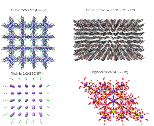
../../_images/SuperCells_CrystalPrep.png — Fig. 9.13 Various generated supercells by employing the orca_crystalprep utility program¶

%crystalprep


#************************
#Read CIF/XYZ
#************************
DoCIF true                #Turn on the cif file reading

#------------------------
#INPUT CIF/XYZa
#------------------------
InputCIF "CeO2.cif"       #The cif file 
#------------------------
#Set Special Tasks
#------------------------

#************************
#Generate SuperCell
#************************
DoSuperCell true           #Turn on the supecell construction
SCDimension "10x10x10"     #Construct a 10x10x10 supercell
DoSymetricSC true          #Construct symmetric supercell 
DoSymmetryOperations true  #Use the buildin Crystallographic database
DoHemiSphereSC true/false  #Build the supecell in cubic or hemisphere fashion
PrintLevel 2
#************************
#Setup Embedding Approach
#************************
DoEmbedding false          #Turn off the Embended Cluster generation

Running this will process the .cif file

*************** ORCA CRYSTALPREP TOOL ************

-------------------------------------------------------------
Reading Information from the provided CIF file: CeO2.cif
-------------------------------------------------------------

------------------------Unit Cell Parameters-----------------
Hermann-Mauguin Space Group:     P1
Space Group ID:                1
Unit Cell Symmetry:                
Unit Cell Volume:            163.40
Unit Cell alpha angle:        90.00
Unit Cell beta angle:         90.00
Unit Cell gamma angle:        90.00
Unit Cell alpha length:       5.467
Unit Cell beta length:        5.467
Unit Cell gamma length:       5.467
Atom   Type  AO    x     y     z    occ   ox
 Ce     0    58 0.000 0.000 0.000  1.00  4.00
 Ce     1    58 0.000 0.500 0.500  1.00  4.00
 Ce     2    58 0.500 0.000 0.500  1.00  4.00
 Ce     3    58 0.500 0.500 0.000  1.00  4.00
 O      4     8 0.250 0.750 0.750  1.00 -2.00
 O      5     8 0.750 0.250 0.250  1.00 -2.00
 O      6     8 0.250 0.250 0.250  1.00 -2.00
 O      7     8 0.750 0.750 0.750  1.00 -2.00
 O      8     8 0.750 0.750 0.250  1.00 -2.00
 O      9     8 0.250 0.250 0.750  1.00 -2.00
 O     10     8 0.750 0.250 0.750  1.00 -2.00
 O     11     8 0.250 0.750 0.250  1.00 -2.00
Done
-------------------------------------------------------------

----------Making a SuperCell with 10x10x10 dimensions-----------
Doing Symmetry Operations ...
Detected   1 Operations for 
Hermann-Mauguin Space Group:     P1
Space Group ID:                  1
Done
Unit Cell:
                  0          1          2    
      0       5.467000   0.000000   0.000000
      1       0.000000   5.467000   0.000000
      2       0.000000   0.000000   5.467000

Transformation Matrix:
                  0          1          2    
      0      54.670000   0.000000   0.000000
      1       0.000000  54.670000   0.000000
      2       0.000000   0.000000  54.670000

-----------------------------
Super Cell Origin:   0,   0,   0
-----------------------------
-----------------------------
The Center of XYZ Coordinates
-----------------------------
2.278, 2.278, 2.278

---------------------------------------------------------------------
Saving xyz file: CeO2.cif_10x10x10.xyz                   ...Done
---------------------------------------------------------------------


*************** ORCA CRYSTALPREP TOOL TERMINATED SUCCESFULLY ************

and will create the 10x10x10 spherical supecell shown in Figure Fig. 9.14 in a cubic (a) or in a hemisphere (b) construction fashion if the DoHemiSphereSC keyword is turned on. Note that while the cubic supercell construction scheme is appropriete for creating embedded clusters to tackle bulk chemical propblems (e.g. computation of the Optical band gaps of semiconductors, [597]). In contrast the hemisphere supercell build option is expected to be very usefull for constructing embedded clusters to tackle surface related problems (e.g. computation of adsorption energies of molecules on surfaces, [811]).

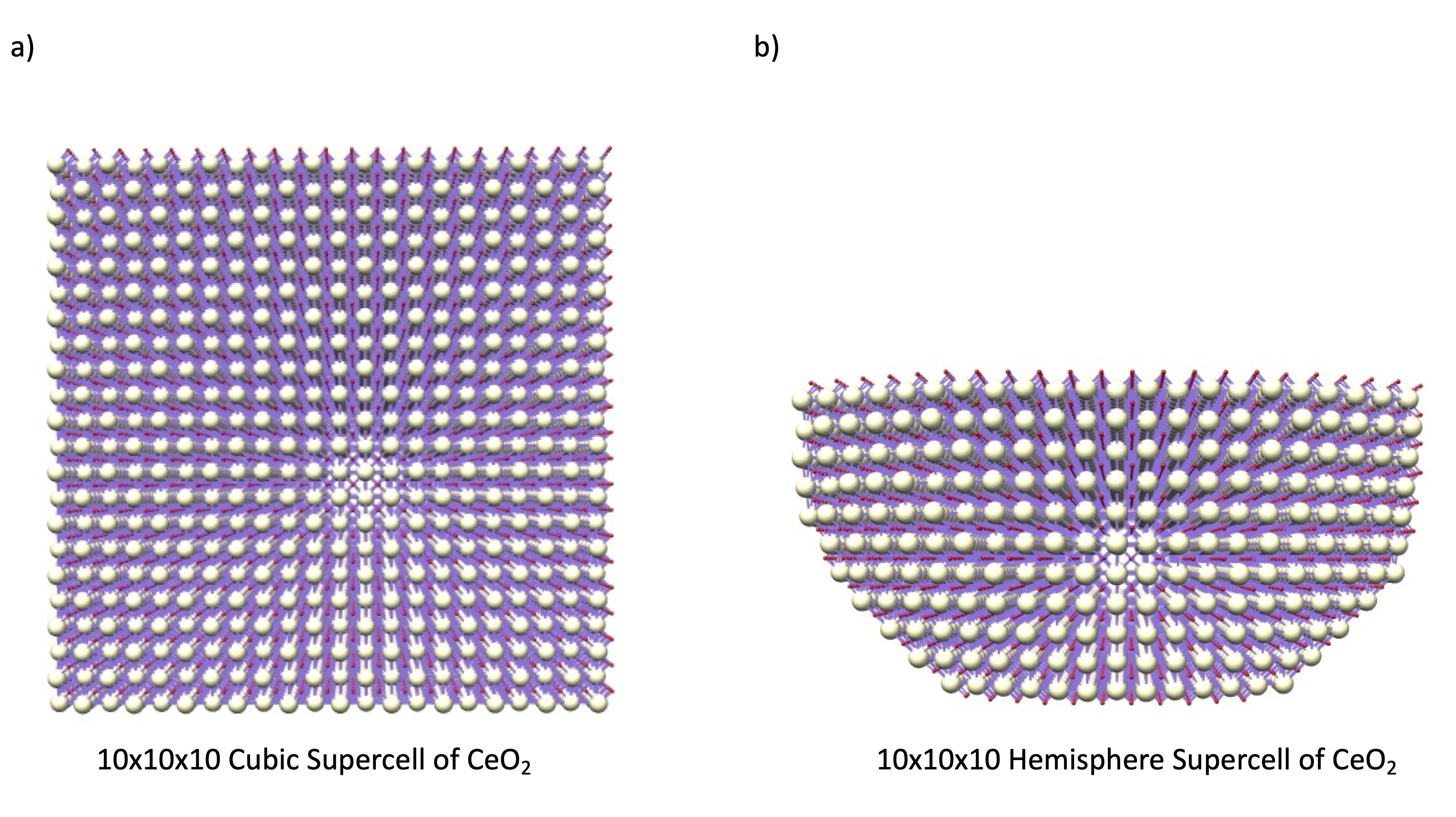
../../_images/CeO2_Supecells_CrystalPrep.png — Fig. 9.14 Cubic (left) versus Hemisphere (right) generated 10x10x10 supercell of CeO2¶

Enable loading of a tailored QC.xyz file

Staring from ORCA 6.1, it is possible to generate and load a tailored QC file directly in orca_crystalprep.

This is achieved by enabling the DoSymetricSC keyword. In this way all generated supercells share the same center. Hence in the case of CeO2, one can generate a 1x1x1 or 2x2x2 minimum supercell and construct/tailor the QC.xyz file (in this case Ce24O64.xyz). In following one can now re-execure the orca_crystalprep by now loading the QC file by setting LoadQCCluster true

%crystalprep


#************************
#Read CIF/XYZ
#************************
DoCIF true

#------------------------
#INPUT CIF/XYZa
#------------------------
InputCIF "CeO2.cif"
InputQCXYZ "Ce24O64.xyz"
LoadQCCluster true
#------------------------
#Set Special Tasks
#------------------------
#SpaceGroupNumber 200

#************************
#Generate SuperCell
#************************
DoSuperCell true
SCDimension "10x10x10"
PrintLevel 2
#************************
#Setup Embedding Approach
#************************
DoEmbedding true
DoSymetricSC true
DoSymmetryOperations true
DoHemiSphereSC true
CellVolumeFraction 0.01
DoLayers true
ECPLayers 3
#------------------------
#Atom Type Charge Spin
#------------------------
NAtomTypes 12
 Ce     0    4.0  0.0
 Ce     1    4.0  0.0
 Ce     2    4.0  0.0
 Ce     3    4.0  0.0
 O      4    -2.0  0.0
 O      5    -2.0  0.0
 O      6    -2.0  0.0
 O      7    -2.0  0.0
 O      8    -2.0  0.0
 O      9    -2.0  0.0
 O     10    -2.0  0.0
 O     11    -2.0  0.0

#************************
#Generate Inputs
#************************
#------------------------
# Simple/IC-QMMM inputs
#------------------------
DoICQMMMInput true

#------------------------
#QCCharge 0
#QCMult 1
#------------------------
end

This will generate the embedded cluster shown in Figure Fig. 9.15 for the tailored QC=\([Ce_{24}O_{48}]^0\) quantum cluster and 3-layers of ECPs.

Note that in this case the different layers to equiop the ECPs and PCs regions are by default generated on the basis of the volume of the chosen QC cluster. In this case it is beneficial to use a small fraction of the unitcell volume defined by CellVolumeFraction 0.01 that can be used as a criterion for the layers generation.

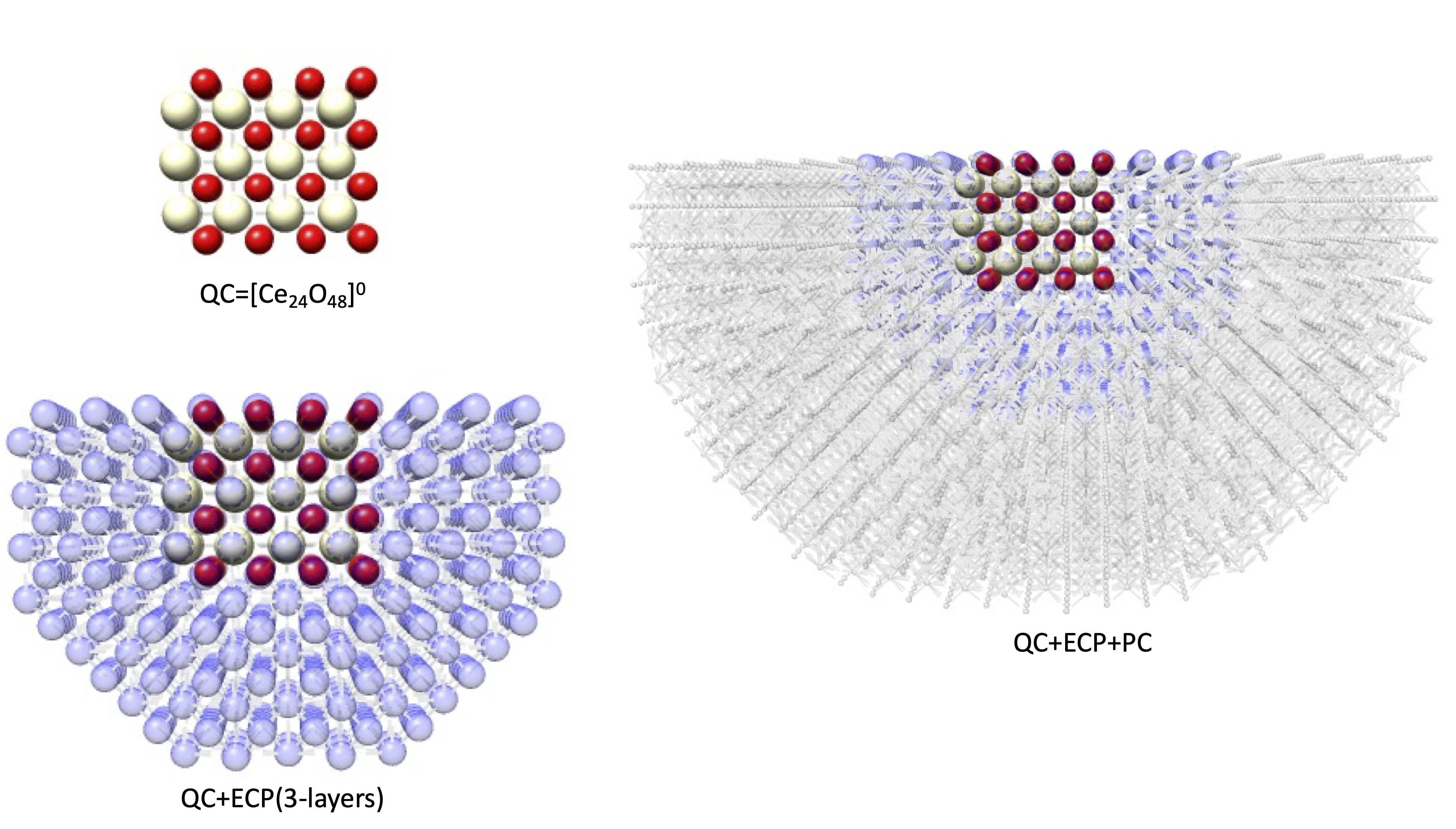
../../_images/CeO2_embedded_cluster.png — Fig. 9.15 CeO2 embedded cluster generated for the QC=\([Ce_{24}O_{48}]^0\) quantum cluster and 3-layers of ECPs¶

In a final step the orca_crystalprep generates the IC-QM/MM input file as

!Ionic-Crystal-QMMM
#Include Method


%qmmm
#--------Define the Cluster---------
ORCAFFFilename= "CeO2.cif_10x10x10.ORCAFF.prms"
Use_QM_InfoFromPDB true
Use_QM3_InfoFromPDB true
ECPLayerECP= "SDD"
#--------Charge Convergence---------
CONV_Charges false
ENFORCETOTALCHARGE true
CHARGE_TOTAL    0
PrintLevel 4
end
#-----------------------------------

*pdbfile 0  1 CeO2.cif_10x10x10.pdb

Note that the information on the QC, ECP and PC regions is read from the generated .pdb file.

Further information on the IC-QM/MM and QM/MM modules in general can be found in section Overview on ORCA’s Multiscale Implementation
Additional details and examples related to the orca_crystalprep tool and the embedding approach are provided in the tutorial “Treating Solids with the Embedding Cluster approach”.