3.16. N-Electron Valence State Perturbation Theory (NEVPT2)
The N-electron valence state perturbation theory (NEVPT) belongs to the family of internally contracted methods and applies to a CASSCF/CAS-CI type reference wave functions. The NEVPT2 methodology developed by Angeli et al exists in two formulations namely the strongly-contracted NEVPT2 (SC-NEVPT2) and the partially contracted NEVPT2 (PC-NEVPT2). [462, 463, 464] Irrespective of the name “partially contracted” coined by Angeli et al, the latter approach employs a fully internally contracted wave function (FIC). Hence, we use the term “FIC-NEVPT2” in place of PC-NEVPT2. NEVPT2 has many desirable properties - among them:
It is intruder state free due to the choice of the Dyall Hamiltonian [465] as the 0th order Hamiltonian.
The 0th order Hamiltonian is diagonal in the perturber space. Therefore no linear equation system needs to be solved.
It is strictly size consistent. The total energy of two non-interacting systems is equal to the sum of two isolated systems.
It is invariant under unitary transformations within the active subspaces.
“strongly contracted”: Perturber functions only interact via their active part. Different subspaces are orthogonal and hence no time is wasted on orthogonalization issues.
“fully internally contracted”: Invariant to rotations of the inactive and virtual subspaces.
Both methods produces energies of similar quality as the CASPT2 approach.[466, 467] The strongly and fully internally contracted NEVPT2 methods are implemented in ORCA, along with a range of approximations that significantly enhance the methodology’s scalability and make it highly attractive for large-scale applications. This includes the ability to handle large basis sets, big molecules, and extended active spaces.
In addition to corrections to the correlation energy, ORCA features a range of spectroscopic properties for NEVPT2, including UV, IR, CD, and MCD spectra, as well as EPR parameters. These properties are computed using the “quasi-degenerate perturbation theory” that is described in section CASSCF Properties. The NEVPT2 corrections enter as “improved diagonal energies” in this formalism. ORCA also offers the multi-state extension (QD-NEVPT2 for the strongly contracted NEVPT2 variant.[468, 469] Here, the reference wave function is revised in the presence of dynamical correlation. For systems, where such reference relaxation is important, the computed spectroscopic properties will improve.
NEVPT2 requires a single keyword on top of a working CASSCF input.
!SC-NEVPT2    # for the strongly contracted NEVPT2
!FIC-NEVPT2   # for the fully internally contracted NEVPT2
!DLPNO-NEVPT2 # for the DLPNO variant of the FIC-NEVPT2
! ...
%casscf ...
Alternatively, the methods are called within the CASSCF block and detailed settings can be adjusted
in the PTSettings subblock.
We will go through some of the detailed setting in the next few
subsections. For historical reasons, a few features, such as the
quasi-degenerate NEVPT2, are only available for the strongly contracted
NEVPT2. As shown elsewhere, the strong contraction is not a good
starting point for linear scaling
approaches.[416] Thus newer additions such as
the DLPNO and the F12 correction rely on the FIC variant.
[470, 471, 472]
Note that ORCA by default employs
the frozen core approximation, which can be disabled with the simple
keyword !NoFrozenCore. A complete description of the frozecore
settings can be found in section
Frozen Core Options.
3.16.1. A simple Example: \(N_2\) Ground State
Let us consider the ground state of the nitrogen molecule as a simple example.
After defining the computational details of our CASSCF calculation, we insert “!SC-NEVPT2” as simple input or
specify “PTMethod SC_NEVPT2” in the %casscf block. Please note the
difference in the two keywords’ spelling: Simple input uses hyphen,
block input uses underscore for technical reasons.
!def2-svp nofrozencore PAtom
%casscf nel  6
        norb 6
        mult 1
        PTMethod SC_NEVPT2 # SC_NEVPT2 for strongly contracted NEVPT2
                           # FIC_NEVPT2 for the fully internally
			   # contracted NEVPT2
                           # DLPNO_NEVPT2 for the FIC-NEVPT2 with DLPNO
                           # DLPNO requires: trafostep RI and an aux basis
end

* xyz 0 1
N       0.0     0.0     0.0
N       0.0     0.0     1.09768
*
For better control over the program flow, it is recommended to split the calculation into two distinct parts. First, converge the CASSCF wave function and inspect the resulting orbitals. Then, in a second step, read the converged orbitals and run the actual NEVPT2 calculation.
---------------------------------------------------------------
                        ORCA-CASSCF
---------------------------------------------------------------

...
PT2-SETTINGS:
A PT2 calculation will be performed on top of the CASSCF wave function (PT2=SC-NEVPT2)
...
---------------------------------------------------------------
                         < NEVPT2  >
---------------------------------------------------------------
...
 ===============================================================
                       NEVPT2 Results
===============================================================
   *********************
    MULT 1, ROOT 0
   *********************

  Class V0_ijab :        dE = -0.017748
  Class Vm1_iab :        dE = -0.023171
  Class Vm2_ab  :        dE = -0.042194
  Class V1_ija  :        dE = -0.006806
  Class V2_ij   :        dE = -0.005056
  Class V0_ia   :        dE = -0.054000
  Class Vm1_a   :        dE = -0.007091
  Class V1_i    :        dE = -0.001963

---------------------------------------------------------------
         Total Energy Correction : dE = -0.15802909
---------------------------------------------------------------
         Zero Order Energy       : E0 = -108.98888640
---------------------------------------------------------------
         Total Energy (E0+dE)    : E  = -109.14691549
---------------------------------------------------------------
Introducing dynamic correlation with the SC-NEVPT2 approach lowers the
energy by 150 mEh. ORCA also prints the contribution of each “excitation
class V” to the first order wave function. We note that in the case of a
single reference wave function corresponding to a CAS(0,0), the V0_ijab
excitation class produces the exact MP2 correlation energy.
In section Example: Breaking Chemical Bonds the
dissociation of the N\(_{2}\) molecule has been investigated with the
CASSCF method. Inserting PTMethod SC_NEVPT2 into the %casscf block
we obtain the NEVPT2 correction as additional information.
! def2-svp nofrozencore
%casscf nel  6
        norb 6
        mult 1
        PTMethod SC_NEVPT2
end

# scanning from the outside to the inside
%paras
	R = 2.5,0.7, 30
end

*xyz 0 1
N 0.0 0.0 0.0
N 0.0 0.0 {R}
*

Fig. 3.37 Potential Energy Surface of the N\(_2\) molecule from CASSCF(6,6) and NEVPT2 calculations (def2-SVP).
All of the options available in CASSCF can in principle be applied to
NEVPT2. Since NEVPT2 is implemented as a submodule of CASSCF, it will
inherit all settings from CASSCF (!tightscf, !UseSym, !RIJCOSX,…).
3.16.2. RI, RIJK and RIJCOSX Approximation
Setting the RI approximation on the CASSCF level, will set the RI options for NEVPT2 respectively. The three index integrals are computed and partially stored on disk. Three index integral with two internal labels are kept in main memory. The two-electron integrals are assembled on the fly. The auxiliary basis must be large enough to fit the integrals appearing in the CASSCF orbital gradient/Hessian and the NEVPT2 part. The auxiliary basis set of the type /J does not suffice here.
%casscf
  ...
  TrafoStep RI   # enable RI approximation in CASSCF and NEVPT2
  PTMethod  SC_NEVPT2 # or the NEVPT2 approach or your choice
end
Additional speedups can be achieved by approximating the Fock operator using
the !RIJCOSX or !RIJK techniques. When using RIJCOSX, an additional auxiliary
basis must be specified for the AuxJ auxiliary basis slot.
For more information on basis set slots, see section Orbital Basis Sets.
#RIJCOSX one-liner
! def2-svp def2/J RIJCOSX def2-svp/C

# Commented out: alternative definition via %basis block
#%basis
#auxJ "def2/J"
#auxC "def2-svp/C"
#end
Whereas the RIJK requires a single auxiliary basis set (AuxJK slot),
that is large enough to fit integrals in the Fock-matrix construction,
orbital gradient/Hessian and the correlation part. In contrast to COSX,
the calculation can also be carried out in conv mode (storing the AO
integrals on disk).
#RIJK one-liner: !conv is recommended.
! def2-svp def2/JK RIJK

# Commented out: Alternative definition via %basis block
#%basis
#auxJK "def2/JK"
#end
The described methodology allows the computation of systems with up to 2000 basis functions. Even larger molecules are accessible in the framework of DLPNO-NEVPT2 described in the next subsection. Several examples can be found in the CASSCF tutorial.
3.16.3. Beyond the RI approximation: DLPNO-NEVPT2
For systems with more than 80 atoms, we recommend the DLPNO-NEVPT2 method,
which combines the DLPNO ansatz with the FIC-NEVPT2 approach.[470]
This method is particularly effective, as it recovers 99.9% of the FIC-NEVPT2 correlation energies, even for large systems.
The input structure for DLPNO-NEVPT2 is similar to that of its parent FIC-NEVPT2 method.
Below, we provide an example input for the Fe(II)-complex depicted in
Fig. 3.38,
where the active space consists of the metal-3d orbitals. The example
takes about 9 hour (including 3 hour for one CASSCF iteration) using 8
cores (2.60GHz Intel E5-2670 CPU) for the calculation to finish. A
detailed description of the DLPNO-NEVPT2 methodology can be found in our
article.[470]. A number of DLPNO specific parameters can
be set in the PTSettings sub-block. The respective keywords are otherwise identical with the
DLPNO Coupled Cluster ansatz described elsewhere in the manual.
The most important parameters are TCutPNO, TCutMKNand TCutDO. However, it is recommended
to use the simple keywords !TightPNO, !NormalPNO or !LoosePNO to adjust the accuracy.
In contrast to the canonical FIC-NEVPT2 method, the DLPNO amplitude equations require the solution of a set of linear equations.
The latter are solved iteratively via a DIIS solver, which comes with its own set of control parameters.
# DLPNO-NEVPT2 calculation for quintet state of FeC72N2H100
!PAL8 def2-TZVP def2/JK
!moread noiter
%moinp "FeC72N2H100.gbw-CASSCF"
%MaxCore 8000
%casscf
  nel 6
  norb 5
  mult 5

  # mandatory for DLPNO-NEVPT2:
  PTMethod DLPNO_NEVPT2  # will automatically set `TrafoStep RI`


  # optional settings reapting the defaults
  PTSettings
    # DLPNO specific settings (see DLPNO-NEVPT2 article):
    TCutPNO      1e-8 # cutoff for PNO occupation numbers
    TCutPNO_Core 1e-2 # cutoff for PNO occupation numbers for core orbitals
    TCutMKN      1e-3 # cutoff for Mulliken populations in the PNO
                      # integral transformation
    TCutDO       1e-2 # cutoff for the sparse map construction of domain
    TCutDOij     1e-5 # cutoff for the differential overlap matrix of ij pairs
                      # in the prescreening step

    # DLPNO DIIS solver settings:
    MaxIter    30    # maximum number of iterations
    MaxDIIS    7     # DIIS max. dimension
    DIISDamp1  0.5   # damping of the residual before DIIS is switched ON
    DIISDamp2  0     # damping of the residual after DIIS is switched ON
    LevelShift 0.2   # LevelShift during update
    LMP2TolE   1e-7  # energy convergence criteria
    LMP2TolR   5e-7  # residual convergence criteria
    LMP2Damp   1.0   # damping for the LMP2 amplitude update

  end
end
*xyz 0 5 FeC72N2H100.xyz
Just like RI-NEVPT2, the calculations requires an auxiliary basis. The
aux-basis should be of /C or /JK type (more accurate). Aside from the
paper of Guo et al,[470] a concise report of
the accuracy can be found in the CASSCF tutorial, where we compute
exchange coupling parameters. Note that in the snippet above, we have
commented out the default setting in the PTSettings sub-block.
As mentioned earlier, the CASSCF step can be accelerated with the RIJK or RIJCOSX approximation. Both options are equally valid for the DLPNO-NEVPT2. The RIJK variant typically produces more accurate results than RIJCOSX. The input file is almost the same as before, except for the keyword line:
# The combination of RIJK with DLPNO-NEVPT2
!PAL8 def2-TZVP def2/JK conv RIJK
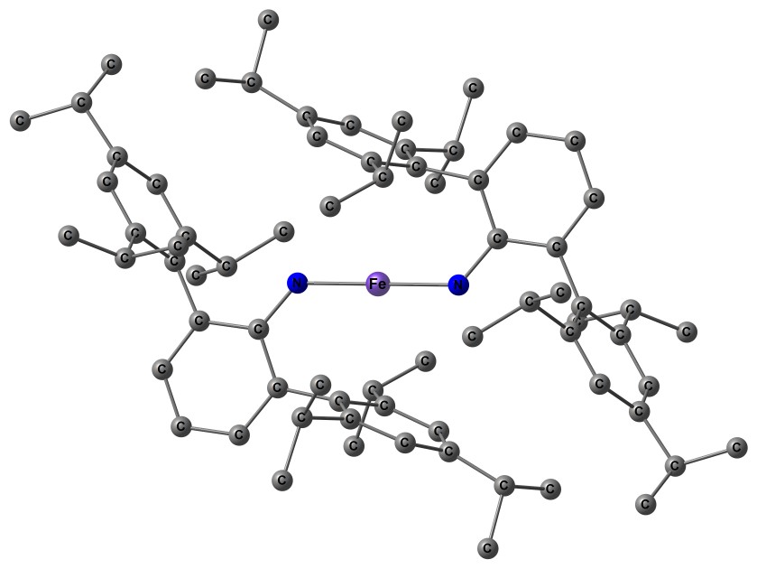
Fig. 3.38 Structure of the FeC\(_{72}\)N\(_{2}\)H\(_{100}\)
3.16.4. Explicit Correlation: NEVPT2-F12 and DLPNO-NEVPT2-F12
Like in the single-reference MP2 theory, the NEVPT2 correlation energy
converges slowly with the basis set. Aside from basis set extrapolation,
the R12/F12 method are popular methods to reach the basis set limit. For
comparison of F12 and extrapolation techniques, we refer to the study of
Liakos et al.[384] ORCA features an F12 correction
for the FIC-NEVPT2 wave function using the RI
approximation.[471] The RI approximation is mandatory
as the involved integrals are expensive. In complete analogy to the
single reference MP2-F12, the input requires an F12 basis, an F12-cabs
basis and a sufficiently large RI basis (/JK or /C). It should be noted, that
the CASSCF wave function itself is also affected by basis set incompleteness. When F12 is invoked, a perturbative correction for
CASSCF reference, denoted as CABS singles correction, is added.[473]
# aug-cc-pvdz/C used as RI basis
 ! cc-pvdz-F12 aug-cc-pvdz/C cc-pvdz-f12-cabs
 %casscf nel 8
         norb 6
         mult 3,1

         # mandatory:
         TrafoStep RI        # RI approximation must be on for F12
         PTMethod FIC_NEVPT2 # FIC-NEVPT2
         PTSettings
           F12 true    # request the F12 correction and CABS singles correction.
         end
 end
 *xyz 0 3
  O      0.0 0.0 0.0
  O      0.0 0.0 1.207
 *
A linear scaling version of NEVPT2-F12, the DLPNO-NEVPT2-F12, allows to
tackle systems with several thousand of basis functions.[471, 472]
With the exception of the DLPNO_NEVPT2 keyword, the input structure is otherwise identical to NEVPT2-F12
method.
# aug-cc-pvdz/C used as RI basis
! cc-pvdz-F12 aug-cc-pvdz/C cc-pvdz-f12-cabs
%casscf nel 8
        norb 6
        mult 3,1

        # mandatory:
        TrafoStep RI           # RI approximation must be on for F12
        PTMethod DLPNO_NEVPT2  # DLPNO variant
        PTSettings
          F12 true             # request the F12 correction and CABS singles correction.
        end
end
*xyz 0 3
 O      0.0 0.0 0.0
 O      0.0 0.0 1.207
*
Note that the DLPNO-NEVPT2-F12 algorithm is unitary invariant with
respect to subspace rotation of inactive and active orbitals. By
tightening the DLPNO truncation thresholds (TCutPNO,TCutDO, TCutCMO and TCutDOij),
the canonical NEVPT2-F12 can be reproduced, even with localized internal and active molecular
orbitals.
3.16.5. Handling of Reduced Density Matrices
NEVPT2 calculations involve the computation of higher order reduced density matrices (RDMs), which can quickly become a major bottleneck for active spaces of CAS(10,10) and larger. Using Dyall’s rank-reduction scheme,[474] the standard implementation involves at most the fourth order reduced density matrix (4-RDM).[464] In contrast, omitting the rank-reduction scheme, the full rank NEVPT2 (FR-NEVPT2) requires the 5-RDM and its contractions.[423] The latter should be used in the context of approximate CAS-CI reference wave functions such as the ICE.
ORCA uses an efficient reformulation of the NEVPT2 method, that avoids the explicit 4-RDM and 5-RDM construction.[475]
The basic idea is similar to a recent development reported by Sokolov and coworkers.[476]
The algorithm requires a memory-intense intermediates, that scales with the number of configuration state functions (CSFs) in the CAS-CI.
With the option D4Step fly, the memory demands are reduced at the expense of computation time omitting the aforementioned intermediate.
%casscf
  ...
  PTMethod     FIC_NEVPT2  # or SC_NEVPT2

  # detailed settings (optional)
  PTSettings
  D4Step efficient # efficient: calling the default RDM handling
                   # fly      : slower but more economic code
                   #
                   # Cu4 : cumulant approximation of the 4-RDM
                   # Cu34: cumulant approximation of the 3-RDM and 4-RDM
  D4TPre 1e-12     # default PS approximation 4-RDM
  D3TPre 1e-14     # default PS approximation 3-RDM
  imaginary 0.0    # imaginary shift (only for FIC-NEVPT2)
end
3.16.5.1. PS Approximation (default)
To accelerate the evaluation of the higher-order RDMs, ORCA uses a prescreening approximation (PS) for the reference wave function.[418]
Only configurations with a weight larger than a specified parameter D4TPre are taken into account. The same reduction is available for the third
order density matrix using the keyword D3TPre. Both parameters can be adjusted within the PTSettings sub-block of the CASSCF module.
The exact NEVPT2 energy is recovered with the parameters set to zero. The approximation is available for all variants of NEVPT2
(SC, FIC and DPLNO-FIC). The default thresholds, D4TPre 1e-12 and D3TPre=1e-14, are chosen very conservative as lowering might lead to false intruder states.[418, 423]
These approximations naturally affect the “configuration RI” as well. In this context, it should be noted that a configuration corresponds to a set of CSFs with identical orbital occupation. For each state the dimension of the CI and and RI space is printed.
  D3 Build          ... CI space truncated: 141 -> 82  CFGs
                    ... RI space truncated: 141 -> 141 CFGs
  D4 Build          ... CI space truncated: 141 -> 82  CFGs
                    ... RI space truncated: 141 -> 141 CFGs
3.16.5.2. Cumulant Approximation (optional)
Large computational savings can be achieved with the cumulant expansion, which have been recently re-evaluated.[418] The results should be treated with care as false intruder states can emerge.[477] In these cases, the imaginary level shift is the only mitigation tool.[478] Note that the imaginary shift is only implemented for FIC-NEVPT2.
PTSettings
  D4Step Cu4    # Cu4  : approximate the 4-RDM
                # Cu34 : approximate the 3-RDM and 4-RDM
  imaginary 0.0 # imaginary shift (only for FIC-NEVPT2)
end
3.16.6. False Intruder States and Imaginary Shift
False intruder states are introduced by crude approximations of the reduced density matrices or the reference wave function.[418, 423] The occurance is highly system-specific. Indications are unreasonable correlation energy contributions from the 1-hole excitation class (denoted as “V_i” or “ITUV”) or the 1-particle excitation class (denoted as “V_a” or “TUVA”), e.g., positive or large correlation energies compared to the 2-hole-2-particle excitation class (denoted as “V_ijab” or “IJAB”). For transparency, ORCA prints warnings when the Koopmans energies or the energy denominators are negative.
...
WARNING: Denominator is negative for DEpsilon ITUV i=2 mu=1 : -344.12813836782095 < 0
WARNING: Denominator is negative for DEpsilon ITUV i=2 mu=2 : -228.47393616112132 < 0
WARNING: Denominator is negative for DEpsilon ITUV i=2 mu=3 : -218.57612632153200 < 0
WARNING: Denominator is negative for DEpsilon ITUV i=2 mu=4 : -127.85082085035380 < 0
Skipped =       126 of          432 LowestEV=-3.843455e+02 ... done in        0.1 sec
 Reached max. number of intruder state warning (5). Thus, warnings were suppressed for
 this class to limit the output!

WARNING: Koopmans matrices have at least one negative eigenvalue (-1.519147e+06)
         Please check your results carefully.
To avoid flooding the output, the number of warnings are limited by MaxWarnings (default=5). When faced with these warnings, it is advised
to inspect the approximations of the reduced density matrices. For example, in the case of the PS approximation, tightening the thresholds (D4TPre=1e-14) should
immediately alleviate the issue. The cumulant approximation in particular is prone to false intruder states and should thus be avoided.
As a last resort, an imaginary shift can be added to mitigate intruder states.[478] Note that imaginary shifts (default=0.0 ) are restricted to the canonical FIC-NEVPT2 implementation.
PTSettings
  imaginary 0.2 # imaginary shift (only for FIC-NEVPT2) . default = 0.0
  MaxWarnings 5 # Max number of denominator warnings before going silent.
end
3.16.7. Large Active Spaces: ICE-NEVPT2
Standard CAS-CI solver can perform routine calculation up to a CAS(14,14) active space. Larger active spaces are accessible with the ICE ansatz.[439]
With a recent extension of the FIC-NEVPT2 methodology, that also allows an ICE reference wave functions, calculation with active spaces up to CAS(34,34) are possible.[455]
As shown in the paper by Guo et al, for an approximate CAS-CI solution, the canonical implementation, that uses Dyall’s rank reduction scheme,
cannot be applied without introducing false intruder states. Hence, for an ICE reference wave function, ORCA defaults to the full-rank
NEVPT2 formulation (FR-NEVPT2), where additional 5-RDM contributions are accounted for. The latter are enabled with CASCI_Approx true.
While the default ICE parameter TVar is designed for the ICE-CASSCF-Iterations, it is less ideal for the NEVPT2 approach. Here, the computation of the higher-order RMDs is a major bottleneck
and not feasible with the same threshold. As demonstrated by Guo et al, a parameter of TVar 1e-7 (=TGen x \(10^{-3}\)) already leads to reasonable results that balance accuracy and efficiency.
Following the reciple from the paper, it is recommended to split the calculation into two parts. First converge the ICE-CASSCF solution with the default parameters and inspect the resulting orbitals.
Then, in a second step, run the FIC-NEVPT2 with a larger TVar reading the converged orbitals from the first step. For these type of calculation, we recommend to use the D4Step fly algorithm as it
avoids memory-intense intermedidates processing the RDMs.
# Starting with converged CASSCF orbitals
!MORead NoIter
%moinp "converged.ice-casscf.gbw"
%casscf
  ...
  # mandatory keywords for ICE-NEVPT2
  CIStep ICE
  PTMethod FIC_NEVPT2
  CI
    TVar 1e-7 # ICE parameter TVar for ICE-NEVPT2 runs.
              # TVar ~ TGen x 1e-3 - this is larger than the default.
  end


  # optional settings (repeating the defaults)
  PTSettings
    D4Step fly        # memory saving algorithm for larger active spaces
    CASCI_Approx true # setting FR-NEVPT2
    D4TPre 0.0        # recommendation: disabling PS approximation.
                      # No benefit from screening here.
    D3TPre 1e-14      # recommendation: default PS approximation for 3-RDM.
  end
3.16.8. Large Active Spaces: DMRG-NEVPT2
An alternative for larger active spaces is offered by the DMRG ansatz. It is possible to run DMRG-NEVPT2 calculations for the FIC-NEVPT2 and SC-NEVPT2 ansatz using the
methodology developed by the Chan group.[479] Here, the reduced density matrices are provided by the BLOCK program.
It should be noted that the latter is platform dependent and several crashes have been reported in the past. For troubleshooting, please contact the BLOCK developers directly.
Aside from the usual DMRG input, the program requires an additional parameter
(nevpt2_MaxM) in the DMRG block.
%casscf
  cistep DMRGCI
  %dmrg
    ...
    nevpt2_MaxM 2000 # (see Note below)
  end
  PTMethod SC_NEVPT2 # or FIC_NEVPT2
end
3.16.9. Selecting or Specific States for NEVPT2
ORCA by default computes all states defined in the CASSCF block input
with the NEVPT2 approach. There are cases, where this is not desired and
the user wants to skip some of these states. The input mask of
SelectedRoots[block] allows to select only few states for the computation,
where “block” refers to numbering of the multiplicity blocks. The enumeration
of blocks and roots starts with 0.
!NEVPT2 ...
%casscf
  ...
  MULT   3,1 # multiplicity block
  NRoots 2,3 # number of roots for the MULT blocks

  # detailed settings (optional) for the PT2 approaches
  PTSettings
    # option to skip the PT2 correction for all states except for the ones
    # specified for a selected multiplicity block and root
    # selectedRoots[block]  = root number counting from 0.
    selectedRoots[1]=0,1 # compute MULT=1 root=0,1 and skip all others.

  end
end
3.16.10. Unrelaxed Densities and Natural Orbitals
For the FIC-NEVPT2 ansatz, it is possible to request state-specific unrelaxed densities
where \(\Psi_I\) refers to NEVPT2 wave function of the I’th state and consists of the zeroth- and first-order wave function
The code is implemented using the ORCA AGE tool-chain.[358]
The exact unrelaxed density requires higher-order reduced density matrices (RDMs) of the the CAS-CI reference wave function.
The latter can be avoided, when the unrelaxed density is approximated at first order using the keyword FirstOrder.
In that case, the expensive second-order contribution
\(\langle 1|E^p_q)|1\rangle\) is omitted.
A cost-effective alternative, that keeps the second-order term, is the cumulant approximation Cu4 and Cu34. Here, the 4-RDM and optionally the 3-RDM themselves
are approximated to accelerate their computation.
The unrelaxed density can be used to generate natural orbitals with the keyword NatOrbs true.
For each state, ORCA stores the resulting orbitals in a separate GBW file with the suffix “.mult.A.root.B.pt2.nat”, where “A” flags its multiplicity and
“B” its root count. In case of !UseSymmetry, the suffix will also include the irreducible representation of the state.
NEVPT2 natural orbital are mandatory for various analysis tools,
for instance the MultiWFN program.
The orbitals can also be used for natural orbital iterations
(!MORead NoIter) or to systematically extend the active space.[480]
%casscf
  ...
  PTMethod     FIC_NEVPT2

  # detailed settings (optional)
  PTSettings
    # densities are disabled by default
    Density Unrelaxed  # unrelaxed density <0+1|E(p,q)|0+1>
            Cu4        # cumulant 4-rdm approximated unrel. density
            Cu34       # cumulant 3/4-rdm approximated unrel. density
            FirstOrder # approximate unrel. density <0|E(p,q)|1>

    NatOrbs True       # produces the natural orbitals (default=False)
  end
end
Note that ORCA repeats the population analysis for each state. With the added keyword
!KeepDens the NEVPT2 density is stored in the density container (.densities file on disk) with the prefix “Tdens-CASNEV”.
The latter can be used to create density plots interactively (see Section
orca_plot).
Below is a snapshot of a typical output:
Unrelaxed Density     ...
Incorizing ADC        ... done in      0.6 sec
Norm <Psi|Psi>        ... done in      0.1 sec (NORM=     1.064186836)
RDM1 <Psi|E|Psi>      ... done in      0.7 sec
Reference Weight      ...     0.939684618
Trace RDM1            ...    20.000000000 (prior correction)

*** Repeating the population analysis with unrelaxed density.
Orbital energies/occupations assumed diagonal. ***
(Note: Temporarily storing unrelaxed densities as cas.scfp)
------------------------------------------------------------------------------
ORCA POPULATION ANALYSIS
------------------------------------------------------------------------------

...
Natural Orbital Occupation Numbers:
...
N[  4] =   1.98812992
N[  5] =   1.98308480
N[  6] =   1.93858508
N[  7] =   1.49303660
N[  8] =   1.49303660
N[  9] =   1.48519842
N[ 10] =   1.48519842
N[ 11] =   0.05922342
N[ 12] =   0.00921465
N[ 13] =   0.00921465
N[ 14] =   0.00794869
N[ 15] =   0.00620254
...
 ===============================================================
 NEVPT2 Results
 ===============================================================
 ...
3.16.11. State-averaged SC-NEVPT2
In the definition of the Dyall Hamiltonian,[465] the CASSCF orbitals are chosen to diagonalize the Fock operator (pseudo-canonicalized). Therefore, using a state-averaged CASSCF wave function, the NEVPT2 procedure involves the construction and diagonalization of the “state-specific” Fock operators and is thus resulting in a unique set of orbitals for each state. This becomes quickly inefficient for large numbers of states or larger molecules since each orbital set implies an integral transformation. This is the default setting for NEVPT2 and is printed in the output
NEVPT2-SETTINGS:
Orbitals      ... canonical for each state
For the SC-NEVPT2, other orbital options can be set using the keyword canonstep.
%casscf
  ...
  # detailed settings (optional)
  PTSettings
  # SC-NEVPT2 specific options
  canonstep      0         # state-averaged orbitals and specific orbital energies
                 canonical # canonical for each state (default)
                 averaged  # state-averaged orbitals and orbital energies
                 relaxed   # 1-step orbital relaxation
                           # and canonical for each state (partially relaxed)
  end
end
The final orbitals of the state-averaged CASSCF diagonalize the
state-averaged Fock operator. Large computational savings can be made if
these orbitals are employed for all of the states. canonstep 0 chooses
orbital energies as diagonal elements of the state-specific Fock
operators. In release versions ORCA 3.0 and older, this has been the
default setting. These options work best if the averaged states are
similar in nature. For SC-NEVPT2, we have implemented two more
canonsteps, which trade accuracy for speed and vice versa.
canonstep averaged is more approximate and employs orbital energies from the
state-averaged calculation. Thus there is no contribution to excitation
energies from the 2-hole-2-particle perturber class (denoted as “V_ijab” or “IJAB”)
at this level of approximation.
If the states under consideration are substantially different, these
approximations will be of poor quality and should be turned off. Better
results can be achieved, if the state-averaged orbitals are partially
relaxed for each state before the actual SC-NEVPT2 calculation.
[481] Often it is not possible to optimize the orbitals
of each excited state separately. Thus, canonstep relaxed will try a single steepest descent
step for each state before running the actual SC-NEVPT2 calculation with
canonicalized orbitals. Optionally, instead of a steepest descent using
an approximate diagonal Hessian, a single Newton-Raphson step can be
made.
%casscf
  ...
  PTMethod SC_NEVPT2
  # detailed settings
  PTSettings
  canonstep relaxed # orbital relaxation for each state
  gstep SOSCF true  # steepest descent step
  NR    false       # Newton-Raphson   step
  end
end
Despite a converged state-averaged calculation, the gradient for the individual states can be surprisingly large. As a consequence, the orbital relaxation may fail, when both methods are outside their convergence radius. ORCA will retry the relaxation with an increased damping. If the orbital update still fails, the program will stick with the initial orbitals. Setting an overall damping manually may help the relaxation procedure.
%casscf
  ...
  PTMethod SC_NEVPT2
  # detailed settings
  PTSettings
    gscaling 0.5 # damp gradient with a pre-factor
  end
end
3.16.12. Quasi-Degenerate SC-NEVPT2
The NEVPT2 approach presented in the previous subsections follows the recipe of “diagonalize and perturb”. The 0th order wave function is determined by the diagonalization of the CAS-CI matrix. The space spanned by the CAS-CI vectors is often referred to as “model space”. The subsequent perturbation theory is constructed based on the assumption that the states under consideration are well described within the model space. Consequently, the first order correction to the wave function \(\Psi^{(1) }_I\) does not affect the composition of the reference state \(\left|I\right\rangle\). Corrections to the wave function and energy arise from the interaction of the reference state with the functions \(\left|k\right\rangle\) of the contributing first order interacting space
This is problematic, when the interaction/mixing of states are falsely described at the CASSCF level. A typical example is the dissociation of lithium fluoride.
!def2-tzvp nevpt2 nofrozencore

%casscf
  nel 2
  norb 2 #Li(2s), F(2pz)
  mult 1
  nroots 2
end

# unrelaxed scan r=3 to r=7
%paras
r = 3,7,200
end

*xyz 0 1
Li 0 0 0
F 0 0 {r}
*
Here, the ground and first excited state of \(\Sigma^+\) should not cross. However, at the NEVPT2 level, an erratic double crossing is observed instead.

Fig. 3.39 SC-NEVPT2 and QD-SC-NEVPT2 Li-F dissociation curves of the ground and first excited states for a CAS(2,2) reference
A re-organizing of the reference states can be introduced in the framework of quasi-degenerate perturbation theory. In practice, an effective Hamiltonian is constructed allowing “off-diagonal” corrections to the second-order energy
Diagonalization of this eff. Hamiltonian yields improved energies and
a rotation matrix (right eigenvectors) that introduces the desired
re-mixing of the reference states. The quasi-degenerate extension to
SC-NEVPT2 [482] can be switched on with the keyword QDType.
%casscf
  ...
  PTMethod SC_NEVPT2     # Must be SC_NEVPT2
  PTSettings
    PrintLevel 1         # default printing

    # mandatory
    QDType QD_VanVleck # QD_VanVleck: Hermitian  eff. Hamiltonian (recommended)
                       # QD_Bloch   : non-Hermitian eff.
                       # 0: disabled (default)

    # optional: compute the QD-Corrected density.
    QDPopulationAnalysis True # Repeat population analysis with the corrected density
    QDNatOrbs            True # Get natural orbitals with the corrected density
  end
end
ORCA will print the eff. Hamiltonian matrix and its eigenvectors at the
end of the calculation for PrintLevel 4.
===============================================================
                      QD-NEVPT2 Results
===============================================================
  *********************
   MULT 1,
  *********************

  Total Hamiltonian to be diagonalized
                  0          1
     0    -107.074594  -0.012574
     1      -0.011748-107.003810

  Right Eigenvectors
                 0          1
    0      -0.987232   0.170171
    1      -0.159292  -0.985414

--------------------------
        ROOT = 0
--------------------------
        Total Energy Correction : dE = -0.25309172934720
        Zero Order Energy       : E0 = -106.82353108218946
        Total Energy (E0+dE)    : E  = -107.07662281153667

--------------------------
        ROOT = 1
--------------------------
        Total Energy Correction : dE = -0.23103459727281
        Zero Order Energy       : E0 = -106.77074682157986
        Total Energy (E0+dE)    : E  = -107.00178141885267
By construction the Hamiltonian is non-Hermitian (QDType QD_Bloch).
Hence, the computation of properties with the revised wave function, e.g.,
expectation values require left- and right eigenvectors. The diagonalization
of the general matrices appearing in the
Bloch formulations may occasionally lead to complex eigenpairs - an undesirable
artifact. Although, the eigenvalues have typically only a small
imaginary component, the results are not reliable and ORCA prints a
warning.
--- complex eigenvalues and eigenvectors
  WARNING! QD-Matrix has eigenvalues with imaginary component! iE(0)=-0.000016
  WARNING! QD-Matrix has eigenvalues with imaginary component! iE(1)=0.000016
The QD_VanVleck option avoids the general eigenvalue decomposition.
The equations are derived from second-order Van Vleck perturbation
theory, which results in a Hermitian effective Hamiltonian.[469] The
methodology is equivalent to the symmetrization of the Bloch
Hamiltonian. The solution is always real and properties are easily
accessible. Thus, QD_VanVleck is the recommended approach in ORCA.
For a more detailed comparison of the different eff. Hamiltonian
theories, we refer to the literature.[483, 484]
In all formulations, the energy denominator in the
quasi-degenerate NEVPT2 is very sensitive to approximations. The
canonicalization options with averaged orbitals and orbitals energies
(canonstep 0/2) have the tendency to lessen the energy denominator. To
avoid artifacts, the calculation is restricted to canonstep 1, where each
state has its own set of orbitals.
If properties are requested within the casscf module, i.e. zero-field splitting, there will be an additional printing with the revised CI vectors and energies.
In addition, with QDPopulationAnalysis true the population analysis is repeated with the
unrelaxed densities using the revised reference wave function. Using the directive !KeepDens
these densities are stored and kept in the density container as “Tdens-CAS-DPDICPT2” together with
a suffix containing the state details (multiplicity and root). Following the ORCA convention, the suffix ends with “.p” and “.r” for densities
and spin-densities respectively. For clarity, we added a snapshot of the density container (“orca_plot jobname.densities”).
Note that properties, such as Mössbauer,
that are processed in orca_prop, will be re-computed with the revised densities, when it is available/allowed.
Index:                                                   Name of Density
------------------------------------------------------------------------
    0:                                                          cas.scfp
    1:                             Tdens-CAS-DPDICPT2MO.mult.1.iroot.0.p
    2:                               Tdens-CAS-DPDICPT2.mult.1.iroot.0.p
    3:                             Tdens-CAS-DPDICPT2MO.mult.1.iroot.1.p
    4:                               Tdens-CAS-DPDICPT2.mult.1.iroot.1.p
    5:                               Tdens-CAS-DPDICPT2.mult.1.iroot.0.r
    6:                               Tdens-CAS-DPDICPT2.mult.1.iroot.1.r
The revised densities can also be used to form natural orbitals setting QDNatorbs true. The resulting
orbitals are stored in a GBW file with the suffix “mult.A.iroot.B.QD-NEVPT2.natorbs”, where “A” denotes the multiplicity
and “B” the root count.
3.16.13. Keywords
NEVPT2 can also be set using the PTMethod keyword in the %casscf block. Beware of the underscore in the keywords using the block input.
Refined settings are adjusted in the PTSettings subblock. The methods require higher order reduced density matrices, which are not implemented
for all of the CISteps. In addition to the default CIStep, ACCCI, ICE and DMRGCI are supported.
%casscf

  # usual CASSCF settings defining the active space and states of interest
  ...
  MULT   3,1 # multiplicity block
  NRoots 2,3 # number of roots for the MULT blocks

  CIStep    ICE     # CSFCI  : default (recommended)
                    # ACCCI  : fast, but memory intense
                    # ICE    : larger active spaces with ICE FIC-NEVPT2
                    # DMRGCI : larger active spaces with DMRG SC-NEVPT2

  TrafoStep RI      # RI approximation for CASSCF and NEVPT2

  # calling the PT2 method of choice
  PTMethod    SC_NEVPT2    # strongly contracted NEVPT2
              FIC_NEVPT2   # fully internally contracted / partially
	                   # contracted NEVPT2
              DLPNO_NEVPT2 # FIC-NEVPT2 using the DLPNO framework for
	                   # large molecules

  # detailed settings (optional) for the PT2 approaches
  PTSettings
    PrintLevel 1      # default printing
    EWIN  -3,1000     # Energy window for the frozencore setting fc_ewin
    NThresh 1e-6      # FIC-NEVPT2 cut off for linear dependencies

    # handling of reduced density matrices:
    D4Step  efficient # efficient: default 4-RDM handling
                      # fly      : memory saving algorithm for larger active spaces
                      # cu4 : cumulant approximation of the 4-RDM
                      # cu34: cumulant approximation of the 3-RDM and 4-RDM
    D4Tpre  1e-12     # PS approximation of the 4-pdm
    D3Tpre  1e-14     # PS approximation of the 3-pdm

    # false intruder state related options:
    TSMallDenom 1e-2 # printing thresh for small denominators
    MaxWarnings  5   # max number of warning before going silent
    imaginary    0.0 # imaginary shift for FIC-NEVPT2

    # option to skip the PT2 correction for all states except for the ones
    # specified for a selected multiplicity block and root
    # selectedRoots[block]  = root number counting from 0.
    selectedRoots[1]=0,1 # compute MULT=1 root=0,1 and skip all others.


    # SC-NEVPT2 specific features:
    QDType    QD_VanVleck      # QD_VanVleck: Van Vleck (recommended)
                               # QD_Bloch: Bloch Hamiltonian
                               # 0: disabled
    QDNatOrbs True             # get revised density and natural orbitals
    QDPopulationAnalysis True  # get revised density and repeat population analysis

    # SC-NEVPT2 state-average orbital canonicalization options:
    CanonStep   canonical # canonical for each state (default)
                averaged  # state-average
                relaxed   # canonical and partially relaxed for each state.
                0         # state-average, but state-specific orbital energies

    # canonstep=relaxed additional control parameters:
    GScaling 0.5          # damping factor for the stepsize
    GStep    NR           # relax with NR
             SOSCF        # relax with SOSCF
             SUPERCI_PT   # relax with perturbation based SuperCI

    # FIC-NEVPT2 specific features:
    F12       true      # add F12 correction  and CABSSingles correction for CASSCF
    Density   unrelaxed # unrelaxed density generated for each state.
    NatOrbs   true      # computes the natural orbitals

    # DLPNO specific settings for expert users (see DLPNO-NEVPT2 article):
    TCutPNO      1e-8 # cutoff for PNO occupation numbers
    TCutPNO_Core 1e-2 # cutoff for PNO occupation numbers for core orbitals
    TCutMKN      1e-3 # cutoff for Mulliken populations in the PNO
                      # integral transformation
    TCutDO       1e-2 # cutoff for the sparse map construction of domain
    TCutDOij     1e-5 # cutoff for the differential overlap matrix of ij
                      # pairs in the Prescreen step
    # DLPNO DIIS solver settings:
    MaxIter    30    # maximum number of iterations
    MaxDIIS    7     # DIIS max. dimension
    DIISDamp1  0.5   # damping of the residual before DIIS is switched ON
    DIISDamp2  0     # damping of the residual after DIIS is switched ON
    LevelShift 0.2   # LevelShift during update
    LMP2Damp   1.0   # damping for the LMP2 amplitude update
    LMP2TolE   1e-7  # energy convergence criteria
    LMP2TolR   5e-7  # residual convergence criteria
  end
end