5.21. Nuclear Magnetic Resonance (NMR) Parameters

5.21.1. NMR Chemical Shifts

NMR chemical shifts at the HF, DFT (standard GGA and hybrid functionals), CASSCF, as well as the RI- and DLPNO-MP2 and double-hybrid DFT levels (see section MP2 Level Magnetic Properties and references therein), plus Coupled Cluster (GIAO-CCSD, GIAO-CCSD(T), see AUTOCI Response Properties via Analytic Derivatives) can be obtained from the EPR/NMR module of ORCA. For the calculation of the NMR shielding tensor the program utilizes Gauge Including Atomic Orbitals (GIAOs - sometimes also referred to as London orbitals). [683, 684, 685] In this approach, field dependent basis functions are introduced, which minimizes the gauge origin dependence and ensures rapid convergence of the results with the one electron basis set. [686] Note that GIAOs are NOT currently available with CASSCF linear response and a gauge origin must be provided in the %eprnmr block (see CASSCF Linear Response). GIAOs for CASSCF response are coming soon to ORCA! A complete list of possible keywords for the eprnmr module can be found in EPRNMR - keywords for magnetic properties.

The use of the chemical shift module is simple:

# Ethanol - Calculation of the NMR chemical shieldings at the HF/SVP level of theory
! RHF SVP Bohrs NMR

* xyz 0 1
C        -1.22692181     0.24709455    -0.00000000
C        -0.01354839    -0.54677253     0.00000000
H        -2.09280406    -0.41333631     0.00000000
H        -1.24962478     0.87541936    -0.88916500
H        -1.24962478     0.87541936     0.88916500
O         1.09961824     0.30226226    -0.00000000
H         0.00915178    -1.17509696     0.88916500
H         0.00915178    -1.17509696    -0.88916500
H         1.89207683    -0.21621566     0.00000000
*

The output for the shieldings contains detailed information about the para- and diamagnetic contribution, the orientation of the tensor, the eigenvalues, its isotropic part etc. For each atom, an output block with this information is given :

--------------
 Nucleus   0C :
 --------------

Diamagnetic contribution to the shielding tensor (ppm) :
           209.647        -10.519         0.000
           -26.601        215.858         0.000
            -0.000          0.000       200.382

Paramagnetic contribution to the shielding tensor (ppm):
            59.273         18.302        -0.000
            13.380          6.063        -0.000
             0.000         -0.000        -2.770

Total shielding tensor (ppm):
           268.920          7.783        -0.000
           -13.220        221.921        -0.000
             0.000          0.000       197.611


 Diagonalized sT*s matrix:

 sDSO           200.382          214.507          210.998  iso=     208.629
 sPSO            -2.770            7.279           58.057  iso=      20.855
        ---------------  ---------------  ---------------
 Total          197.611          221.786          269.055  iso=     229.484

Note that all units are given in ppm and the chemical shieldings given are absolute shieldings (see below). At the end of the atom blocks, a summary is given with the isotropic shieldings and the anisotropy [687] for each nucleus:

Nucleus  Element    Isotropic     Anisotropy
  -------  -------  ------------   ------------
      0       C          229.484         59.356
      1       C          227.642         62.878
      2       H           56.015         12.469
      3       H           55.460         15.284
      4       H           55.460         15.284
      5       O          334.125        110.616
      6       H           47.337         27.101
      7       H           47.337         27.101
      8       H           64.252         32.114

Thus, the absolute, isotropic shielding for the \(^{13}\)C nuclei are predicted to be 229.5 and 227.6 ppm and for \(^{17}\)O it is 334.1 ppm. While basis set convergence using GIAOs is rapid and smooth, it is still recommended to do NMR calculations with basis sets including tight exponents, such as the purpose-built pcSseg-\(n\). However, TZVPP or QZVP should be sufficient in most cases. [688, 689]

An important thing to note is that in order to compare to experiment, a standard molecule for the type of nucleus of interest has to be chosen. In experiment, NMR chemical shifts are usually determined relative to a standard, for example either CH\(_{4}\) or TMS for proton shifts. Hence, the shieldings for the molecule of interest and a given standard molecule are calculated, and the relative shieldigs are obtained by subtraction of the reference value from the computed value. It is of course important that the reference and target calculations have been done with the same basis set and functional. This also helps to benefit from error cancellation if the standard is chosen appropriately (one option is even to consider an “internal standard” - that is to use for example the \(^{13}\)C shielding of a methyl group inside the compound of interest as reference).

Let us consider an example - propionic acid (CH\(_3\)-CH\(_2\)COOH). In databases like the AIST (http://sdbs.db.aist.go.jp) the \(^{13}\)C spectrum in CDCl\(_3\) can be found. The chemical shifts are given as \(\delta_1\) = 8.9 ppm, \(\delta_2\) = 27.6 ppm, \(\delta_3\) = 181.5 ppm. While intuition already tells us that the carbon of the carboxylic acid group should be shielded the least and hence shifted to lower fields (larger \(\delta\) values), let’s look at what calculations at the HF, BP86 and B3LYP level of theory using the SVP and the TZVPP basis sets yield:

method	\(\sigma_1\)	\(\sigma_2\)	\(\sigma_3\)
HF/SVP	191.7	176.6	23.7
HF/TZVPP	183.5	167.1	9.7
B86/SVP	181.9	165.8	26.5
B86/TZVPP	174.7	155.5	7.6
B3LYP/SVP	181.8	165.8	22.9
B3LYP/TZVPP	173.9	155.0	2.9

Looking at these results, we can observe several things - first of all, the dramatic effect of using too small basis sets, which yields differences of more than 10 ppm. Second, the results obviously change a lot upon inclusion of electron correlation by DFT and are functional dependent. Last but not least, these values have nothing in common with the experimental ones (they change in the wrong order), as the calculation yields absolute shieldings like in the table above, but the experimental ones are relative shifts, in this case relative to TMS.

In order to obtain the relative shifts, we calculate the shieldings \(\sigma_{TMS}\) of the standard molecule (TMS HF/TZVPP: 194.1 ppm, BP86/TZVPP: 184.8 ppm, B3LYP/TZVPP: 184.3 ppm) and by using \(\delta_{mol} = \sigma_{ref} - \sigma_{mol}\) we can evaluate the chemical shifts (in ppm) and directly compare to experiment:

method	\(\delta_1\)	\(\delta_2\)	\(\delta_3\)
HF/TZVPP	10.6	27.0	184.4
B86/TZVPP	10.1	29.3	177.2
B3LYP/TZVPP	10.4	29.3	181.4
Exp.	8.9	27.6	181.5

A few notes on the GIAO implementation in ORCA are in order. The use of GIAOs lead to some fairly complex molecular one- and two-electron integrals and a number of extra terms on the right hand side of the coupled-perturbed SCF equations. The two-electron contributions in particular can be time consuming to calculate. Thus, the RIJK, RIJDX, and RIJCOSX approximations were implemented and tested.[690] By default, the approximation used for the SCF is also applied to the GIAO integrals, but the latter can be changed using the GIAO_2el keyword in the eprnmr input block (see section EPRNMR - keywords for magnetic properties). Note that, while the default COSX grids are typically sufficiently accurate for chemical shifts, the use of defgrid3 is recommended for special cases or post-HF calculations.

The user can finely control for which nuclei the shifts are calculated (although this will not reduce the computational cost very much, which is dominated by the CP-SCF equations for the magnetic field). This works in exactly the same way as for the hyperfine and quadrupole couplings described in the next section. For example:

! B3LYP def2-TZVP TightSCF 

* int 0 1
C  0 0 0  0 0 0
C  1 0 0  1.35 0 0
H  1 2 0  1.1 120 0
H  1 2 3  1.1 120 180
H  2 1 3  1.1 120 0
H  2 1 3  1.1 120 180
*

%eprnmr  
  Ori    = GIAO
  Nuclei = all C { shift }
  Nuclei = all H { shift }
  end

NMR chemical shifts are also implemented in combination with implicit solvent models, hence the NMR keyword can be combined with the CPCM input block. Note that for calculations including implicit solvent, it is highly recommended to also optimize the geometries using the same model. Regardless, explicit solvent–solute interactions observable in NMR (e.g. H-bonds), cannot be modelled with such a model: solvent molecules must be included explicitly in the calculation.

5.21.2. NMR Spin-Spin Coupling Constants

The indirect spin-spin coupling constants observed in NMR spectra of molecules in solution consist of four contributions: The diamagnetic spin orbit term:

(5.94)\[\hat{H}_{DSO}=\frac{1}{2} \sum_{ikl} \frac{ (\vec{M}_k \times \vec{r}_{ik})(\vec{M}_l \times \vec{r}_{il}) }{r_{ik}^3 ~ r_{il}^3} \]

The paramagnetic spin orbit term:

(5.95)\[\hat{H}_{PSO}=\sum_{ik}\frac{\vec{M}_k ~ \vec{l}_{ik} }{r_{ik}^3} \]

The Fermi contact term:

(5.96)\[\hat{H}_{FC}=\frac{8 ~ \pi}{3}\sum_{ik}\delta(r_i-r_k) ~ \mathbf{m}_k \]

And the spin dipole term:

(5.97)\[\hat{H}_{SD}=\sum_{ik} \mathbf{m}_k^T ~ \frac{3 ~ \mathbf{r}_{ik} ~ \mathbf{r}_{ik}^{~T}-r_{ik}^2 }{ r_{ik}^5} ~ \mathbf{s}_{i} \]

While the Fermi contact term is usually the most significant, all contributions can be computed at the HF and DFT level of theory using ORCA. For this purpose, the keyword ssall has to be invoked in the eprnmr input block, while each of the four terms can be requested using ssdso, sspso, ssfc, and sssd, respectively. For example:

! PBE0 pcJ-1 

*xyz 0 1 
O 0.00000        0.00000        0.11779
H 0.00000        0.75545       -0.47116
H 0.00000       -0.75545       -0.47116
*

%eprnmr
 Nuclei = all O { ssall }
 Nuclei = all H { ssfc, sssd }
end

Results will be given in Hz. Note that the default isotopes used might not be the ones desired for the calculation of NMR properties, so it is recommended to define the corresponding isotopes using the ist flag. It is possible to also print the reduced coupling constants \(K\) (in units of \(10^{19}\cdot\mathrm T\cdot \mathrm J^{-2}\)), which are independent of the nuclear isotopes, using the flag PrintReducedCoupling=True.

The CP-SCF equations must be solved for one of the nuclei in each pair and are the bottleneck of the computation. Therefore, spin-spin coupling constants are calculated only between nuclei within a certain distance of eachother (5 Ångstrom by default). The latter can be changed using the SpinSpinRThresh keyword.

If mulitple nuclides are requested, it is also possible to select only certain element pairs (e.g. only C–H and H–H, without C–C) using the SpinSpinElemPairs keyword. Analogously, the SpinSpinAtomPairs keyword selects the actual pairs of nuclei to consider. The union of the latter two options is used to reduce the selection made using the Nuclei input, after which SpinSpinRThresh is applied.

Here is another example illustrating these additional options:

! B3LYP EPR-II

* xyz 0 1 
C     -1.226922    0.247095   -0.000000
C     -0.013548   -0.546773    0.000000
H     -2.092804   -0.413336    0.000000
H     -1.249625    0.875419   -0.889165
H     -1.249625    0.875419    0.889165
O      1.099618    0.302262   -0.000000
H      0.009152   -1.175097    0.889165
H      0.009152   -1.175097   -0.889165
H      1.892077   -0.216216    0.000000
* 

%eprnmr 
  nuclei = all C { ssall, ist = 13 };
  nuclei = all H { ssall, ist = 1  }; 
  nuclei = all O { ssall, ist = 17 }; 
  PrintReducedCoupling true
  SpinSpinRThresh 3.0 # Angstrom
  SpinSpinElemPairs {C C} {O *} # "*" means any element
  SpinSpinAtomPairs {8 *}       # indices start from 0

  # Final selection:
  # C 0 - C 1 
  # C 0 - O 5 
  # C 1 - O 5 
  # C 1 - H 8 
  # H 3 - O 5 
  # H 4 - O 5 
  # O 5 - H 6 
  # O 5 - H 7 
  # O 5 - H 8 
  # H 6 - H 8 
  # H 7 - H 8 
end 

5.21.3. Simulating NMR Spectra

From the computed NMR shieldings and spin-spin coupling constants, the coupled NMR spectra can be simulated. The most typical NMR experiments are decoupled \(^{13}C\) and coupled \(^1H\) spectra, so we will focus on these here. For simulating a full NMR spectrum, we will use ethyl crotonate as an example, and three steps are required: 1) computation of the spin-spin coupling constants, 2) computation of the chemcial shieldings and 3) simulation of the spectrum using a spin-Hamiltonian formalism. Note that these steps can be carried out independently and different levels of theory can be used for shieldings and couplings and the order of steps 1 and 2 doesn’t matter.

Furthermore, if the spectra are to be simulated with TMS as reference, the shieldings for TMS are required (the hydrogen and carbon values in this case are 31.77 and 188.10 ppm, respectively). Here is the input for the calculation for the coupling constants, which is named ethylcrotonate_sscc.inp:

! PBE pcJ-3 autoaux tightscf  

*xyzfile 0 1 ethylcrotonate.xyz

%eprnmr
 Nuclei = all H {ssall}
end

The spin-spin coupling constants will be stored in the file ethylcrotonate_sscc.property.txt, which the simulation of the NMR spectrum will need to read. The NMR shieldings and will be computed in the next step, for which the input ethylcrotonate_nmr.inp looks like this:

!TPSS pcSseg-3 autoaux tightscf NMR  

*xyzfile 0 1 ethylcrotonate.xyz

The final NMR spectrum simulation is carried out using orca_nmrspectrum, which requires a separate input file ethylcrotonate.nmrspec which looks like this (note the required final END statement):

NMRShieldingFile = "ethylcrotonate_nmr"   #property file for shieldings
NMRCouplingFile  = "ethylcrotonate_sscc"  #property file for couplings
NMRSpecFreq = 80.00                       #spectrometer freq [MHz] (default 400)
PrintLevel = 0                            #PrintLevel for debugging info
NMRCoal = 1.0                             #threshold for merged lines [Hz] (default 1)
NMRREF[1] 31.77                           #shielding for 1H reference [ppm]
NMRREF[6] 188.10                          #shielding for 13C reference [ppm]
NMREquiv                                  #lists of NMR-equivalent nuclei
1 {13 14 15} end                          #H 13,14,15 are equivalent (methyl)
2 {16 17} end                             #H 16 and 17 equivalent (ethyl)
3 {8 10 11} end                           #H 8,10,11 again equivalent methyl
end                                       #end equiv nucl block
END                                       #essential end of input

and contains the following keywords:
NMRShieldingFile and NMRCouplingFile denote the .property.txt files from which the shielding tensors and coupling constants will be read by the NMR spectrum module. If this line is not given, the program will exepect the shieldings or couplings in the property file of the current calculation.

NMRSpecFreq The NMR spectrometer frequency in MHz is decisive for the looks of the spectrum as shieldings are given in ppm and couplings are given in Hz. Default is 400 MHz.

NMRCoal If two lines are closer than this threshold (given in Hz) then the module will coalesce the lines to one line with double intensity. Default it 1 Hz.

NMRREF[X] Reference value for the absolute shielding of element X used in the relative shifts of the simulated spectrum. Typically, these are the absolute shielding values from a separate calculation of TMS, for example, and will be zero ppm in the simulated spectrum.

NMREquiv The user has to specify groups of NMR equivalent nuclei. These are typically atoms which interchange on the NMR timescale, like methyl group protons. The shieldings and couplings will be averaged for each group specified by the user.

with this input, orca_nmrspectrum is called with two arguments, the first one is a gbw file which contains all informations about the molecule, typically this is the gbw file of the nmr or the sscc calculation, and the name of the input file given above:

orca_nmrspectrum ethylcrotonate_nmr.gbw ethylcrotonate.nmrspec > output

If this calculation is carried out, the NMR spectrum module will read the files
ethylcrotonate_sscc.property.txt and ethylcrotonate_nmr.property.txt, extract the shieldings and couplings, average the equivalent nuclei and set up an effective NMR spin Hamiltonian for each nucleus:

(5.98)\[{H}_{NMR}(p,q)= \sigma_{p} \delta_{pq} + J_{pq} I_p I_q. \]

Caution

This includes all nuclei this nuclear spin couples to and should not contain too many spins (see SpinSpinRThres), as the spin Hamiltonian for each atom and the nuclei it couples to is diagonalized brute force. Afterwards, all spin excitations are accumulated and merged into the final spectrum for each element. For ethyl crotonate the NMR spectrum output looks like this:

----------------------------------------------------- 
 NMR Peaks for atom type 1, ref value  31.7700 ppm : 
----------------------------------------------------- 
Atom   shift[ppm]   rel.intensity  
   8        2.34    9.00 
   8        2.36    9.00 
   8        2.25    9.00 
   8        2.27    9.00 
   9        6.34    1.00 
   9        6.36    3.00 
   9        6.38    3.00 
   9        6.41    1.00 
   9        6.14    1.00 
   9        6.16    3.00 
   9        6.19    3.00 
   9        6.21    1.00 
  12        7.95    1.00 
  12        7.85    3.00 
  12        7.75    4.00 
  12        7.65    4.00 
  12        7.56    3.00 
  12        7.47    1.00
  13        1.71    9.00 
  13        1.61   18.00 
  13        1.52    9.00 
  16        4.56    4.00 
  16        4.46   12.00 
  16        4.37   12.00 
  16        4.27    4.00 

----------------------------------------------------- 
 NMR Peaks for atom type 6, ref value 188.1000 ppm : 
----------------------------------------------------- 
Atom   shift[ppm]   rel.intensity  
   2       25.70    1.00 
   3      155.15    1.00 
   4       19.96    1.00 
   5       68.91    1.00 
   6      174.39    1.00 
   7      130.29    1.00 

----------------------------------------------------- 
 NMR Peaks for atom type 8, ref value 104.8826 ppm : 
----------------------------------------------------- 
Atom   shift[ppm]   rel.intensity  
   0        0.00    5.00 
   1      149.74    5.00

The first column denotes the atom number of the nucleus the signal arises from, the second column denotes the line position in ppm and the third line denotes the relative intensity of the signal. For oxygen, no reference value was given, so the program will autmatically set the lowest value obtained in the calculation as reference value.

Using gnuplot, for example, to plot the spectrum, the following plots for \(^{13}C\) and \(^1H\) are obtained [1] :

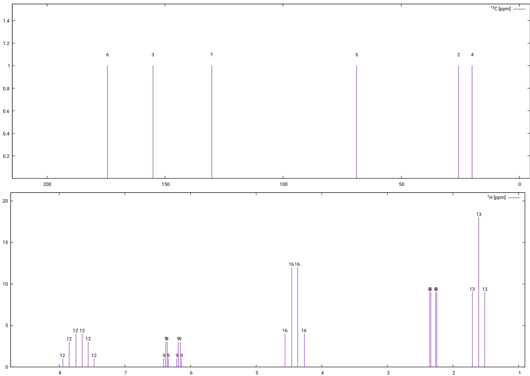
Fig. 5.62 Simulated \(^13C\) (top) and 1H (bottom) NMR spectra. Note that as only HH couplings have been computed, the spectra do not include any CH couplings and the carbon spectrum is also uncoupled.

This makes comparison to experiment and assessment of the computed parameters much easier, however, it is not as advanced as other codes and does not, for example, take conformational degrees of freedom etc. into account. Note that the corresponding property files can also be modified to tinker with the computed shieldings and couplings.

5.21.4. Visualizing shielding tensors using orca_plot

For the visualization it is recommended to perform an ORCA NMR calculation such that the corresponding gbw and density files required by orca_plot are generted by using the !keepdens keyword along with !NMR. If orca_plot is called in the interactive mode by specifying orca_plot myjob.gbw -i (note that myjob.gbw, myjob.densities and myjob.property.txt have to be in this directory), then following 1 - type of plot and choosing 17 - shielding tensor, confirming the name of the property file and then choosing 11 - Generate the plot will generate a .cube file with shielding tensors depicted as ellipsoids at the corrsponding nuclei. These can be plotted for example using Avogadro, isosurface values of around 1.0 and somewhat denser grids for the cube file (like 100x100x100) are recommended. A typical plot for CF\(_3\)SCH\(_3\) generated with Avogadro looks like this [2]:

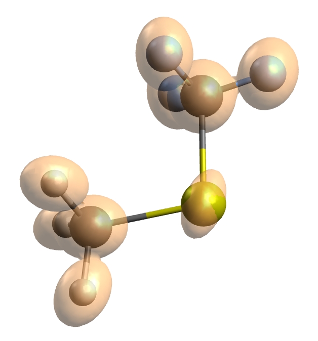
Fig. 5.63 The shielding tensors of each atom in CF3SCH3 have been plotted as ellipsoids (a,b and c axis equivalent to the normalized principle axes of the shielding tensors) at the given nuclei.

5.21.5. Nucleus-independent chemical shielding

Aromaticity is a fundamental concept in chemistry and much attention has been payed to its analysis in quantum chemistry. One possibility to gain insight into aromaticity is to sample the ring current effect in NMR close to the \(\pi\)-system. As this is not done by inspecting the chemical shielding of any of the atoms, this quantity is called nucleus independent chemical shielding (NICS). Usually, a “dummy” atom is placed in the center of the ring and/or at some distance away from it. In ORCA, one needs to use a ghost atom, e.g. “H:” to ensure that the program generates DFT or COSX grid points in the region on interest. For technical reasons, this atom must also have at least one basis function, which can be set with NewGTO. An s-function with a sufficiently large exponent will not overlap with any other basis function in the molecule and will thus have no effect on the results, but only satisfy the technical requirement (note that the extra grid points may change some of the calculation results by increasing the accuracy of the numerical integration). If RI is used, a dummy fitting function must also be added to the AuxJ, AuxJK, and/or AuxC basis set. A typical input for benzene looks like this:

! TightSCF NMR PBE def2-TZVP RI def2/J
* gzmt 0 1
    H:                              NewGTO S 1 1 1e6 1 end NewAuxJGTO S 1 1 2e6 1 end
    H:  1   1                       NewGTO S 1 1 1e6 1 end NewAuxJGTO S 1 1 2e6 1 end
    C   1   1.39    2   90
    C   1   1.39    2   90  3   60
    C   1   1.39    2   90  4   60
    C   1   1.39    2   90  5   60
    C   1   1.39    2   90  3  -60
    C   1   1.39    2   90  6   60
    H   3   1.09    4   120 1   180
    H   4   1.09    3   120 1   180
    H   5   1.09    4   120 1   180
    H   6   1.09    5   120 1   180
    H   7   1.09    3   120 1   180
    H   8   1.09    7   120 1   180
*

5.21.6. Shielding tensor orbital decomposition

It is possible to decompose the NMR shielding tensor into orbital- or orbital pair contributions. One such option is the Natural Chemical Shielding analysis (see Section Natural Chemical Shielding Analysis (NCS)), while another is presented here. The shielding tensor for nucleus \(A\) can be exactly decomposed as follows:

\[\begin{split}\begin{aligned} \boldsymbol{\sigma}^A &= \sum_{p}\left( \boldsymbol{\sigma}^{A,\text{para} }_p + \boldsymbol{\sigma}^{A,\text{dia} }_p \right)\\ \boldsymbol{\sigma}^{A,\text{para/dia} }_i &= \boldsymbol{\sigma}^{A,\text{para/dia} }_{ii} +\frac{1}{2}\sum_{j\ne i}\left( \boldsymbol{\sigma}^{A,\text{para/dia} }_{ij} + \boldsymbol{\sigma}^{A,\text{para/dia} }_{ji} \right) +\sum_{a}\left( \boldsymbol{\sigma}^{A,\text{para/dia} }_{ia} + \boldsymbol{\sigma}^{A,\text{para/dia} }_{ai} \right)\\ \boldsymbol{\sigma}^{A,\text{para/dia} }_a &= \boldsymbol{\sigma}^{A,\text{para/dia} }_{aa} +\frac{1}{2}\sum_{b\ne a}\left( \boldsymbol{\sigma}^{A,\text{para/dia} }_{ab} + \boldsymbol{\sigma}^{A,\text{para/dia} }_{ba} \right) \\ \boldsymbol{\sigma}^{A,\text{para} }_{pq} &= D^\mathbf{B}_{pq} h^{\mathbf{M}_A}_{pq} \\ \boldsymbol{\sigma}^{A,\text{dia} }_{pq} &= D_{pq} h^{\mathbf{B,M}_A}_{pq} \\ D_{pq} &= \sum_{\mu\nu\kappa\lambda} c_{\mu p} S_{\mu\nu} D_{\nu\kappa} S_{\kappa\lambda} c_{\lambda q} \\ D^\mathbf{B}_{pq} &= \sum_{\mu\nu\kappa\lambda} c_{\mu p} S_{\mu\nu} D^\mathbf{B}_{\nu\kappa} S_{\kappa\lambda} c_{\lambda q} \\ h^{\mathbf{M}_A}_{pq} &= \sum_{\mu\nu} c_{\mu p} h^{\mathbf{M}_A}_{\mu\nu} c_{\nu q} \\ h^{\mathbf{B,M}_A}_{pq} &= \sum_{\mu\nu} c_{\mu p} h^{\mathbf{B,M}_A}_{\mu\nu} c_{\nu q}\end{aligned}\end{split}\]

Note that for SCF methods (HF or DFT), \(\boldsymbol{\sigma}^{A,\text{para/dia} }_a=0\). To request the analysis, a valid GBW file must be given with the keyword LocOrbGBW, which can contain any orthonormal MOs in the same basis, e.g. canonical or localized, although the decomposition above assumes that the Brillouin condition is fulfilled and may be misleading if performed over NBOs for example. Orbital contributions over 0.01 ppm are printed – this is currently not user-configurable. The separate orbital pair contributions can also be printed using Printlevel=3. The following example input calculates HF and RI-MP2 shieldings for formaldehyde and decomposes them over Pipek–Mezey localized orbitals (note that the virtual orbitals are likely not well localized - AHFB would be better suited there). The second sub-calculation just prints the LMOs for convenient visualization with Avogadro.

! RI-MP2 NMR TightSCF RIJK pcSseg-1 cc-pwCVDZ/C def2/JK
%base "H2CO_NMR_PM"
%loc
  LocMet PM    # Pipek-Mezey localization
  Occ    true  # localize both occupied
  Virt   true  # and virtual orbitals (better use AHFB for these!)
  T_core -1e5  # including the core
end
%eprnmr
  PrintLevel 3 # print orbital pair contributions (lots of output!)
  LocOrbGBW "H2CO_NMR_PM.loc" # use these orbitals
end
!xyzfile       # store the coordinates
*gzmt 0 1
  O 
  C 1 1.2078
  H 2 1.1161 1 121.74
  H 2 1.1161 1 121.74 3 180
*
# read the localized orbitals and print them in the output
# for easy visualization with Avogadro
$new_job
! HF pcSseg-1 NoRI MORead NoIter PrintBasis PrintMOs
%moinp "H2CO_NMR_PM.loc"
*xyzfile 0 1 H2CO_NMR_PM.xyz

5.21.7. Treatment of Tau in Meta-GGA Functionals

For GIAO-based calculations with meta-GGAs, different options are available for the kinetic energy density \(\tau\). The current-independent \(\tau_0\) is not gauge-invariant. Ignoring the terms, which produce the gauge-dependence, leads to an ad-hoc gauge-invariant treatment (this was the default up to ORCA 5). A gauge-invariant definition \(\tau_\text{MS}\), containing an explicit dependence on the magnetic field, was proposed by Maximoff and Scuseria.[691] However, this ansatz produces unphysical paramagnetic contributions to the shielding tensor.[692] The last option, introduced by Dobson,[693] is gauge-invariant but requires the solution of the CP-SCF equations, even for pure density functionals. For a discussion and comparison of these alternatives see refs [694] (in the context of TDDFT) and [692, 695] (in the context of NMR shielding). Note that the calculated shieldings can differ substantially between the different approaches! Some other electronic structure programs use the MS ansatz by default, so be careful when comparing results between different codes. In ORCA the treatment of \(\tau\) in GIAO-based calculations is chosed as follows

%eprnmr	
  Tau 0      # gauge-variant
      GI     # ad-hoc gauge-invariant
      MS     # field-dependent, gauge-invariant version of Maximoff and Scuseria
      Dobson # (default) current density-dependent, gauge-invariant version of Dobson
  end

5.21.8. Cartesian Index Conventions for EPR and NMR Tensors

The NMR shielding tensor \(\boldsymbol{\sigma}\) and the EPR \(g\) and \(A\) tensors are in general nonsymmetric matrices. It is therefore important to know the conventions used with regard to their cartesian indices. These conventions stipulate the order of the vector–matrix–vector multiplications in the respective spin Hamiltonians. Unless stated otherwise, ORCA adopts the following conventions:

For the NMR shielding tensor the nuclear Zeeman Hamiltonian assumes the form:

\[H_{\!I} = -g_N\beta_N\mathbf{B}(\mathbf{1} - \boldsymbol{\sigma})\mathbf{I},\]

where \(\mathbf{B}\) is the applied magnetic field vector.

For the EPR \(g\) and \(A\) tensors the EPR spin Hamiltonian assumes the form:

(5.99)\[ H_S = \beta_e \mathbf{B}\mathbf{g}\mathbf{S} + \mathbf{S}\mathbf{A}\mathbf{I}. \]

5.21.9. EPRNMR - keywords for magnetic properties

Calculation of EPR and NMR response properties can be requested in the %eprnmr input block. The individual flags are given below.

%eprnmr
  # Calculate the g-tensor using CP-KS theory
  gtensor true
  # Calculate and print one- and two-electron contributions to the g-tensor
  gtensor_1el2el true

  # Calculate the D-tensor
  DTensor so      # spin orbit part
          ss      # spin-spin part
          ssandso # both parts
  DSOC    qro     # quasi-restricted method; must be done with the keyword !uno
          pk      # Pederson-Khanna method.
                  # NOTE: both approximations are only valid for
                  # pure functionals (no HF exchange)
          cp      # coupled-perturbed method (default)
          cvw     # van W\"ullen method
  DSS     direct  # directly use the canonical orbitals for the spin density
          uno     # use spin density from UNOs

  PrintLevel n    # Amount of output (default 2)

  # whether to calculate and print the Euler angles via `orca_euler` if the
  # calculation of the g-tensor or the D-tensor is requested
  PrintEuler false

  # For the solution of the CP-SCF equations:
  Solver   Pople  # Pople solver (default)
           CG     # conjugate gradient
           DIIS   # DIIS type solver
  MaxIter  64     # maximum number of iterations
  MaxDIIS  10     # max. number of DIIS vectors (only DIIS)
  Tol      1e-3   # convergence tolerance
  LevelShift 0.05 # level shift for DIIS (ignored otherwise)

  Ori     CenterOfElCharge  # center of electronic charge
          CenterOfNucCharge # center of nuclear charge
          CenterOfSpinDens	# center of spin density
          CenterOfMass      # center of mass
          GIAO              # use the GIAO formalism (default)
          N                 # number of the atom to put the origin
          X,Y,Z             # explicit position of the origin 
                            # in coordinate input units (Angstrom by default)

  # Calculate the NMR shielding tensor
  NMRShielding 1 # for chosen nuclei - specified with the Nuclei keyword
               2 # for all nuclei - equivalent to the 'NMR' simple input keyword

  # treatment of 1-electron integrals in the RHS of the CPSCF equations
  giao_1el = giao_1el_analytic   # analytical, default
             giao_1el_numeric    # numerical - for testing only

  # treatment of 2-electron integrals in the RHS of the CPSCF equations
  # various options for combination of approximations in Coulomb (J) and
  # exact (HF) exchange (K) part. The default is the same as used for the SCF.
  giao_2el = giao_2el_rijk        # RIJK approximation
             giao_2el_same_as_scf # use same scheme as in SCF
             giao_2el_analytic    # fully analytical
             giao_2el_rijonx      # RIJ approximation with analytical K
             giao_2el_cosjonx     # COSJ approximation with analytical K
             giao_2el_rijcosx     # RIJ approximation with COSX approximation
             giao_2el_cosjx       # COSJ approximation with COSX apprxomation
             giao_2el_exactjcosx  # exact J with COSX approximation
             giao_2el_exactjrik   # exact J with RIK approximation
             
  # for g-tensor calculations using the SOMF-operator for the SOC 
  # treatment, the 2-electron contribution to the GIAO terms can be 
  # computed as well, but they take much more time and usually do not
  # contribute significantly and therefore are disabled by default
  do_giao_soc2el false

  # treatment of tau in meta-GGA DFT - see above
  Tau = Dobson # (default) Other options: 0, MS, GI

  # use effective nuclear charges for the gauge correction to the A-tensor
  # (this makes sense if an effective 1-electron SOC operator is used)
  hfcgaugecorrection_zeff true

  # calculate diamagnetic spin-orbit (DSO) integrals needed for the gauge
  # correction to the A-tensor numerically (faster than the analytical way)
  hfcgaugecorrection_numeric true

  # Grid settings for the above: <0 means to use the DFT grid setting
  hfcgaugecorrection_angulargrid -1
  hfcgaugecorrection_intacc      -1
  hfcgaugecorrection_prunegrid   -1
  hfcgaugecorrection_bfcutoff    -1
  hfcgaugecorrection_wcutoff     -1

  Nuclei = all type { flags }
    # Calculate nuclear properties. Here the properties
    # for all nuclei of "type" are calculated ("type" is
    # an element name, for example Cu.)
    # Flags can be the following:
    #   aiso  - calculate the isotropic part of the HFC
    #   adip  - calculate the dipolar part of the HFC
    #   aorb  - 2nd order contribution to the HFC from SOC
    #   fgrad - calculate the electric field gradient
    #   rho   - calculate the electron density at the
    #           nucleus
    #   shift - NMR shielding tensor (orbital contribution)
    #   srot  - spin-rotation tensor
    #   ssdso - spin-spin coupling constants, diamagnetic spin orbit term 
    #   sspso - spin-spin coupling constants, paramagnetic spin orbit term
    #   ssfc  - spin-spin coupling constants, Fermi contact term
    #   sssd  - spin-spin coupling constants, spin dipole term 
    #   ssall - spin-spin coupling constants, calculate all above contributions 

  # In addition you can change several parameters
  # e.g. for a different isotope.
  Nuclei = all N { PPP=39.1, QQQ=0.5, III=1.0 };
      # PPP   - the HFC proportionality factor for this nucleus
      #         = ge*gN*betaE*betaN
      # QQQ   - the quadrupole moment for this nucleus
      # III   - the spin for this nucleus
      # ist   - isotope
      # ssgn  - nuclear g-factor for spin-spin coupling
      #         and spin-rotation constants (overrides ist)

  # For example:
  # calculates the hyperfine coupling for all nitrogen atoms
  Nuclei = all N { aiso, adip, fgrad, rho};

  # calculates the spin-spin coupling constants for all carbon atoms
  # assuming all carbon atoms are 13C
  Nuclei = all C { ssall, ist = 13};

  # You can also calculate properties for individual atoms
  # as in the following example:
  Nuclei = 1,5,8 { aiso, adip};

  # NOTE: Counting starts with atom 1!
  # WARNING: All the nuclei, mentioned in one line 
  # as above will be assigned the same parameters !

  # For spin-spin coupling constants, a distance threshold is 
  # applied in the eprnmr block to restrict the number of couplings
  # to be computed, given in Angstroms:
  SpinSpinRThresh 5.0 # default

  # Coupling can be restricted to certain element pairs
  # (if they are added to the "Nuclei" list and are within RThresh).
  # The syntax accepts multiple pairs of element symbols or
  # atomic numbers or "*" as a wildcard
  SpinSpinElemPairs {C C} {H *} {6 7} # default is {* *}, i.e. all

  # Similarly, coupling can be restricted to certain atom pairs
  # (if they are added to the "Nuclei" list and are within RThresh).
  # The syntax accepts multiple pairs of indices (starting at 0!)
  # or "*" as a wildcard
  SpinSpinAtomPairs {1 0} {5 *} # default is {* *}, i.e. all

  # whether to print reduced spin-spin coupling constants
  PrintReducedCoupling false

  end

5.22. Paramagnetic NMR Shielding Tensors

For systems with spin \(S>0\), the nuclear shielding contains a contribution which arises from the paramagnetism of the unpaired electrons.[3] This contribution is temperature-dependent and is called the “paramagnetic shielding” (\(\boldsymbol{\sigma}^\mathrm{p}\)). It adds to the temperature-indendent contribution to the shielding, also called the “orbital” contribution:

\[\boldsymbol{\sigma} = \boldsymbol{\sigma}^\mathrm{orb} + \boldsymbol{\sigma}^\mathrm{p}.\]

ORCA currently supports the calculation of \(\boldsymbol{\sigma}^\mathrm{p}\) for systems whose paramagnetism can be described by the effective EPR spin Hamiltonian

(5.100)\[ H_S = \mathbf{S}\mathbf{D}\mathbf{S} + \beta_e \mathbf{B}\mathbf{g}\mathbf{S} + \mathbf{S}\mathbf{A}\mathbf{I}. \]

The theoretical background can be found in Refs. [696, 697]. We reproduce here the main equations.

For a spin state described by Eq. (5.100), the paramagnetic shielding tensor is given by

(5.101)\[ \boldsymbol{\sigma}^\mathrm{p} = -\frac{\beta_e S(S+1) }{g_N\beta_N 3kT} \mathbf{g}\mathbf{Z}\mathbf{A}, \]

where \(\mathbf{Z}\) is a dimensionless \(3\times3\) matrix which is determined by the ZFS and the temperature, as follows: Diagonalization of the ZFS Hamiltonian \(\mathbf{S}\mathbf{D}\mathbf{S}\) yields energy levels \(E_\lambda\) and eigenstates \(|S\lambda a\rangle\), where \(a\) labels degenerate states if \(E_\lambda\) is degenerate. Then \(\mathbf{Z}\) is defined as (\(i,j=x,y,z\))

\[\begin{split}\begin{gathered} Z_{ij} = \frac{3}{S(S+1) }\frac{1}{Q_0} \sum_\lambda e^{-E_\lambda/kT} \Bigg[\sum_{a,a'}\langle S\lambda a|S_i|S\lambda a'\rangle\langle S\lambda a'|S_j|S\lambda a\rangle\\ +2kT\sum_{\lambda'\neq\lambda}\sum_{a,a'} \frac{\langle S\lambda a|S_i|S\lambda' a'\rangle\langle S\lambda' a'|S_j|S\lambda a\rangle }{E_{\lambda'}-E_\lambda} \Bigg],\end{gathered}\end{split}\]

where \(Q_0 = \sum_{\lambda',a} e^{-E_\lambda/kT}\) denotes the partition function. An important property of the \(\mathbf{Z}\) matrix as defined above is that it goes to the identity matrix as \(\mathbf{D}/kT\) goes to zero.

The orbital part of the shielding, \(\boldsymbol{\sigma}^\mathrm{orb}\), is calculated in the same manner as for closed-shell molecules. It is available in ORCA for the unrestricted HF and DFT methods and for MP2 (see Section MP2 Level Magnetic Properties for more information on the latter).

The orca_pnmr tool uses Eq. (5.101) to calculate \(\boldsymbol{\sigma}^\mathrm{p}\). Usage of orca_pnmr is described in Section orca_pnmr.

5.23. Spin-rotation Constants

Spin-rotation constant calculations are implemented using perturbation-dependent atomic orbitals following [699]. As given in eq. 34 of that reference, the spin-rotation tensor of nucleus \(K\), \(\mathbf{M}_K\), is related to the nuclear shielding tensor computed with GIAOs, \(\boldsymbol{\sigma}_K^\text{GIAO}\), and the diamagnetic part of the shielding tensor with the gauge origin set at that nucleus, \(\boldsymbol{\sigma}_K^\text{dia}(\mathbf{R}_K)\):

\[ \mathbf{M}_K = 2 \gamma_K \left( \boldsymbol{\sigma}_K^\text{GIAO} - \boldsymbol{\sigma}_K^\text{dia}(\mathbf{R}_K) \right) \mathbf{I}^{-1} - \mathbf{M}_K^\text{nuc} \]

where \(\mathbf{M}_K^\text{nuc}\) is the nuclear component (given in eq. 14 of the reference), \(\mathbf{I}\) is the inertia tensor, and \(\gamma_K\) is the nuclear magnetogyric ratio. Accordingly, upon requesting spin-rotation constants, ORCA automatically computes the NMR shieldings with GIAOs as well. Note that a complete list of possible keywords for the eprnmr module can be found in EPRNMR - keywords for magnetic properties.

The following input shows an example calculation of \(\mathbf{M}(^{17}\text{O})\) in H₂¹²C¹⁷O:

! HF pcSseg-1 Mass2016 Bohrs
*xyz 0 1
     O        -0.00000000    -0.00000000     1.13863731 M=16.999131
     C        -0.00000000    -0.00000000    -1.14131773 M=12.0
     H        -0.00000000     1.76770755    -2.24076285
     H         0.00000000    -1.76770755    -2.24076285
*
%eprnmr
  Nuclei = all O {srot, ist=17}
end

Note

• The magnetogyric ratio used can be changed either by choosing the correct isotope via ist, or by providing the nuclear g-factor directly via ssgn.

• The masses used to compute the inertia tensor are independent of the chosen isotopes! The example above requests atomic masses of the most abundant isotope (via the Mass2016 keyword) and explicitly specifies those of ¹²C (which is the default) and ¹⁷O.

---

[1]

The basic plot options for using gnuplot are plot "mydata" using 2:3 w i, "mydata" using 2:3:1 with labels

[2]

the same scheme can be applied to visualize polarisability tensors in the molecular framework using orca_plot.

[3]

For a comprehensive review on paramagnetic NMR, see e.g. [698].