5.36. Local Energy Decomposition
The DLPNO-CCSD(T) method provides very accurate relative energies and allows to successfully predict many chemical phenomena. In order to facilitate the interpretation of coupled cluster results, we have developed the Local Energy Decomposition (LED) analysis [775, 776, 777], which permits to divide the total DLPNO-CCSD(T) energy (including the reference energy) into physically meaningful contributions. A practical guide to the LED scheme is reported in Section Section 5.36.1 and Section Section 5.36.2.
Examples of applications of this scheme can be found in Ref. [778, 779, 780, 781, 782, 783].
As a word of caution we emphasize that only the total energy is an observable and its decomposition is, to some extent, arbitrary. Nevertheless, the LED analysis appears to be physically well grounded and logical to us, it is straightforward to apply and comes typically at a negligible computational cost compared to DLPNO-CCSD(T) calculations. Starting from ORCA 4.1, the LED scheme is available for both closed shell and open shell calculations. The code has also been made parallel and more efficient.
The LED scheme makes no assumption about the strength of the intermolecular interaction and hence it remains valid and consistent over the entire potential energy surface. Alternative schemes, such as the popular symmetry adapted perturbation theory, are perturbative in nature and hence are best applied to weakly interacting systems.
The idea of the LED analysis is rather simple. In local correlation methods occupied orbitals are localized and can be readily assigned to pre-defined fragments in the molecule. The same can be done for the correlation energy in terms of pair correlation energies that refer to pairs of occupied orbitals. In this way, both the correlation and the reference energy can be decomposed into intra- and interfragment contributions. The fragmentation is user defined. An arbitrary number of fragments can be defined. In the case that more than 2 fragments are defined, the interfragment interaction is printed for each fragment pair.
A very important feature of the LED scheme is the possibility to distinguish between dispersive and non-dispersive parts of the DLPNO-CCSD(T) correlation energy. In brief, we exploit the fact that each CCSD pair correlation energy contribution can be expressed as a sum of double excitations from pairs of occupied orbitals into the virtual space. As in the DLPNO-CCSD(T) scheme the virtual space is spanned by Pair Natural Orbitals (PNOs) that are essentially local, the entire correlation energy can be decomposed into double excitations types, depending on where occupied and virtual orbitals are localized. For each pair of fragments, the sum of all excitations corresponding to the interaction of instantaneous local dipoles located on different fragments defines the so called “London dispersion” attraction between the two fragments in the LED framework.
For a system of two fragments, one can use as a reference point the geometrically and electronically relaxed fragments that constitute the interacting super-molecule. Relative to this reference state, the binding energy between the fragments can be written as:
where \(\Delta E_{geo-prep}\) is the energy needed to distort the fragments from their equilibrium configuration to the interacting geometry (also called “strain” in other energy decomposition schemes). The \(\Delta E_{el-prep}^{ref.}\) term represents the electronic preparation energy and describes how much energy is necessary to bring the fragments into the electronic structure that is optimal for interaction. \(E_{exch}^{ref.}\) is the inter-fragment exchange interaction (it always gives a binding contribution in our formalism) and \(E_{elstat}^{ref.}\) is the electrostatic energy interaction between the distorted electronic clouds of the fragments. The sum of these terms gives the Hatree-Fock energy in the closed shell case and the energy of the QRO determinant in the open shell case. Finally, the correlation energy is decomposed into dispersive \(E^{C-CCSD}_{dispersion}\) and non-dispersive \(\Delta E^{C-CCSD}_{non-dispersion}\) contributions plus a triples correction term to the interaction energy \(\Delta E^{C-(T) }_{int}\).
The \(E^{C-CCSD}_{dispersion}\) term contains the London dispersion contribution from the strong pairs described above plus the interfragment component of the weak pairs, which is essentially dispersive in nature. The \(\Delta E^{C-CCSD}_{non-dispersion}\) correlation term serves to correct the contributions to the binding energy approximately included in the reference energy, e.g it counteracts the overpolarization typical of the HF method. It contains the so called charge transfer excitations from the strong pairs \(E_{C-SP}^{CT(X\rightarrow Y) } + E_{C-SP}^{CT(X\leftarrow Y) }\), which represent the sum of all double excitation contributions that do not conserve the charge within each fragment. Moreover, the non-dispersive term also includes the electronic preparation from strong (\(\Delta E_{el-prep}^{C-SP}\)) and weak (\(\Delta E_{el-prep}^{C-WP}\)) pairs. Finally, \(\Delta E^{C-(T) }_{int}\) represents the triples correction contribution to the interaction energy between the fragments. In the LED scheme, this term can be further decomposed into intra- and interfragment components. This can be useful, for example, to estimate the London dispersion contribution from the triples correction term, as suggested in Ref. [779].
“Local Energy Decomposition” (LED) analysis [775, 776, 777] is a tool for obtaining insights into the nature of intermolecular interactions by decomposing the DLPNO-CCSD(T) energy into physically meaningful contributions. For instance, this approach can be used to decompose the DLPNO-CCSD(T) interaction energy between a pair of interacting fragments, as detailed in Section Section 5.36. A useful comparison of this scheme with alternative ways of decomposing interaction energies is reported in Ref. [784, 785, 786].
5.36.1. Closed shell LED
LED decomposes separately the reference (Hartree-Fock) and correlation parts of the DLPNO-CCSD(T) energy. By default, the decomposition of the reference energy makes use of the RI-JK approximation. An RIJCOSX variant, which is much more efficient and has a much more favorable scaling for large systems, is also available, as detailed in section Section 5.36.8, and in [784].
Note
For weakly interacting systems, !TightPNO settings are typically recommended.
5.36.1.1. Basic Usage
All that is required to obtain this decomposition in ORCA is to define
the fragments and specify the
!LED keyword in the simple input line.
dlpno-ccsd(t) cc-pvdz cc-pvdz/c cc-pvtz/jk LED
5.36.1.2. Example
As an example, the interaction of H\(_2\)O with the carbene CH\(_2\) at the PBE0-D3/def2-TZVP-optimized geometry can be analyzed within the LED framework using the following input file:
! dlpno-ccsd(t) cc-pvdz cc-pvdz/c cc-pvtz/jk rijk verytightscf TightPNO LED

*xyz 0 1
  C(1)      0.16044643459993      0.10093183177121      0.22603351276210
  H(1)      1.04516129053973     -0.06834886965353     -0.41865951747519
  H(1)     -0.12579332868173      1.14737893892114      0.00305818518771
  O(2)     -1.48285705560792     -1.31933824653169      2.29891474420047
  H(2)     -0.91417368674145     -0.93085192992263      1.60917234463506
  H(2)     -1.15648922489703     -2.21246650333085      2.42094328175662
*
The corresponding output file is reported below. The DLPNO-CCSD(T) energy components are printed out in different parts of the output as follows:
E(0)                                       ...   -114.913309038
E(CORR)(corrected)                         ...     -0.350582526
Triples Correction (T)                     ...     -0.006098691
E(CCSD(T))                                 ...   -115.269990255
At the beginning of the LED part of the output, information on the fragments and the assignment of localized MOs to fragments are provided.
 ===========================================================
         LOCAL ENERGY DECOMPOSITION FOR DLPNO-CC METHODS
 ===========================================================

Maximum Iterations for the Localization .. 600
Tolerance for the Localization          ..  1.00e-06
Number of fragments = 2
Fragment  1:  0 1 2
Fragment  2:  3 4 5

Populations of internal orbitals onto Fragments:
   0:      1.000    0.000  assigned to fragment   1
   1:      0.000    1.000  assigned to fragment   2
   2:      1.022    0.008  assigned to fragment   1
   3:      0.001    0.999  assigned to fragment   2
   4:      0.001    0.999  assigned to fragment   2
   5:      1.018    0.000  assigned to fragment   1
   6:      1.019    0.000  assigned to fragment   1
   7:      0.006    1.013  assigned to fragment   2
   8:      0.000    1.016  assigned to fragment   2
The decomposition of the Hatree-Fock energy into intra- and inter-fragment contributions follows. It is based on the localization of the occupied orbitals.
----------------------------------------
REFERENCE ENERGY E(0) DECOMPOSITION (Eh)
----------------------------------------

Nuclear repulsion     =      28.952049689006
One electron energy   =    -214.430545074583 (T=  114.825132245389, V= -329.255677319972)
Two electron energy   =      70.565186347093 (J=   71.658914661909, K=   -1.093728314816)
                        --------------------
Total energy          =    -114.913309038483
Consistency check     =    -114.913309038483 (sum of intra- and inter-fragment energies)

Kinetic energy        =     114.825132245389
Potential energy      =    -229.738441283873
                        --------------------
Virial ratio          =       2.000767922417

-------------------------------------------
INTRA-FRAGMENT REF. ENERGY FOR FRAGMENT   1
-------------------------------------------

Nuclear repulsion     =      6.037208782874
One electron energy   =    -63.553431032444 (T=   38.870491681225, V= -102.423922713669)
Two electron energy   =     18.675214766985 (J=   18.935443192480, K=   -0.260228425495)
                        -------------------
Total energy          =    -38.841007482585

Kinetic energy        =     38.870491681225
Potential energy      =    -77.711499163811
                        -------------------
Virial ratio          =      1.999241476056


-------------------------------------------
INTRA-FRAGMENT REF. ENERGY FOR FRAGMENT   2
-------------------------------------------

Nuclear repulsion     =      9.103529882464
One electron energy   =   -123.025684625357 (T=   75.954640564164, V= -198.980325189521)
Two electron energy   =     37.916781954190 (J=   38.739989208810, K=   -0.823207254620)
                        -------------------
Total energy          =    -76.005372788703

Kinetic energy        =     75.954640564164
Potential energy      =   -151.960013352867
                        -------------------
Virial ratio          =      2.000667927913


----------------------------------------------------
INTER-FRAGMENT REF. ENERGY FOR FRAGMENTs   2 AND   1
----------------------------------------------------

Nuclear repulsion     =    13.811311023669
Nuclear attraction    =   -27.851429416782
Coulomb repulsion     =    13.983482260618
                        ------------------
Sum of electrostatics =    -0.056636132494 (  -35.540 kcal/mol)

Two electron exchange =    -0.010292634701 (   -6.459 kcal/mol)
                        ------------------
Total REF. interaction =   -0.066928767195 (  -41.998 kcal/mol)


Sum of INTRA-fragment REF. energies  =      -114.846380271288
Sum of INTER-fragment REF. energies  =        -0.066928767195
                                      ---------------------
Total REF. energy                    =      -114.913309038483
Afterwards, a first decomposition of the correlation energy is carried out. The different energy contributions to the correlation energy (strong pairs, weak pairs and triples correction) are decomposed into intra- and inter-fragment contributions. This decomposition is carried out based on the localization of the occupied orbitals.
--------------------------------
CORRELATION ENERGY DECOMPOSITION
--------------------------------


--------------------------------------------------
INTER- vs INTRA-FRAGMENT CORRELATION ENERGIES (Eh)
--------------------------------------------------

                              Fragment   1         Fragment   2
                         -----------------  -------------------
Intra strong pairs         -0.136594658271     -0.209970193798  sum=   -0.346564852069
Intra triples              -0.002692277706     -0.002842791265  sum=   -0.005535068971
Intra weak pairs           -0.000001573694     -0.000002311734  sum=   -0.000003885429
Singles contribution        0.000000000611      0.000000001058  sum=    0.000000001669
                         -----------------  -------------------
                           -0.139288509061     -0.212815295738  sum=   -0.352103804799


Interaction correlation for Fragments   2 and   1:
--------------------------------------------------
Inter strong pairs               -0.003998018810 (   -2.509 kcal/mol)
Inter triples                    -0.000563621667 (   -0.354 kcal/mol)
Inter weak pairs                 -0.000015771468 (   -0.010 kcal/mol)
                          ----------------------
Total interaction                -0.004577411945 (   -2.872 kcal/mol)


Sum of INTRA-fragment correlation energies  =        -0.352103804799
Sum of INTER-fragment correlation energies  =        -0.004577411945
                                              ---------------------
Total correlation energy                    =        -0.356681216744
Afterwards, a summary with the decomposition of the total energy (reference energy + correlation) into intra- and inter-fragment contributions is printed.
--------------------------------------------
INTER- vs INTRA-FRAGMENT TOTAL ENERGIES (Eh)
--------------------------------------------

                                Fragment   1         Fragment   2
                         -------------------  -------------------
Intra REF. energy           -38.841007482585    -76.005372788703  sum=  -114.846380271288
Intra Correlation energy     -0.139288509061     -0.212815295738  sum=    -0.352103804799
                         -------------------  -------------------
                            -38.980295991646    -76.218188084441  sum=  -115.198484076087


Interaction of Fragments   2 and   1:
-------------------------------------
Interfragment reference          -0.066928767195 (  -41.998 kcal/mol)
Interfragment correlation        -0.004577411945 (   -2.872 kcal/mol)
                          ----------------------
Total interaction                -0.071506179140 (  -44.871 kcal/mol)


Sum of INTRA-fragment total energies        =      -115.198484076087
Sum of INTER-fragment total energies        =        -0.071506179140
                                              ---------------------
Total energy                                =      -115.269990255228
Hence, the decomposition reported above allows one to decompose all the components of the DLPNO-CCSD(T) energy into intrafragment and interfragment contributions simply based on the localization of the occupied orbitals. In order to convert the intra-fragment energy components into contributions to the binding energy, single point energy calculations must be carried out on the isolated monomers, frozen in the geometry they have in the adduct, and the corresponding terms must be subtracted. Note that one can also include the geometrical deformation energy (also called “strain”) by simply computing the energy of the geometrically relaxed fragments (see Section Section 5.36 for further information).
For the DLPNO-CCSD strong pairs, which typically dominate the correlation energy, a more sophisticated decomposition, based on the localization of both occupied orbitals and PNOs, is also carried out and printed. Accordingly, the correlation energy from the strong pairs is divided into intra-fragment, dispersion and charge transfer components. Note that, due to the charge transfer excitations, the resulting intra-fragment contributions (shown below) differ from the ones obtained above.
---------------------------------------------
DECOMPOSITION OF CCSD STRONG PAIRS INTO
    DOUBLE EXCITATION TYPES (Eh)
---------------------------------------------

Foster-Boys localization is used for localizing PNOs

Intra fragment contributions:
INTRA Fragment 1                       -0.132849855
INTRA Fragment 2                       -0.209493798

Charge transfer contributions:
Charge Transfer 1 to 2                 -0.005725404
Charge Transfer 2 to 1                 -0.000899609

Dispersion contributions:
Dispersion  2,1                        -0.001594204

Singles contributions:
Singles energy                          0.000000002
More detailed information into the terms reported above can be found in
Section Section 5.36 and in Ref. [775].
All the individual double excitations contributions constituting the
terms reported above can be printed by specifying “printlevel 3” in the
%mdci block. Finally, a summary with the most important terms of the
DLPNO-CCSD energy, which are typically discussed in standard
applications, is printed.
-------------------------------------------------
FINAL SUMMARY DLPNO-CCSD ENERGY DECOMPOSITION (Eh)
-------------------------------------------------

Intrafragment REF. energy:
Intra fragment   1 (REF.)              -38.841007483
Intra fragment   2 (REF.)              -76.005372789

Interaction of fragments  2 and  1:
Electrostatics (REF.)                  -0.056636132
Exchange (REF.)                        -0.010292635
Dispersion (strong pairs)              -0.001594204
Dispersion (weak pairs)                -0.000015771

Sum of non dispersive correlation terms:
Non dispersion (strong pairs)          -0.348968665
Non dispersion (weak pairs)            -0.000003885
Note that the “Non dispersion” terms include all the components of the correlation energy except London dispersion [778, 785]. For the strong pairs, “Non dispersion” includes charge transfer, intrafragment double excitations and singles contributions. For the weak pairs, it corresponds to the intrafragment correlation contribution. In order to convert the non dispersion correlation components into contributions to the binding energy, single point energy calculations must be carried out on the isolated monomers.
5.36.2. Example: LED analysis of intermolecular interactions
The water-carbene example from the previous section will be used to demonstrate how to analyze intermolecular interactions between two fragments using the LED decomposition (note that all energies are given in a.u. if not denoted otherwise). As often done in practical applications, we will be using geometries optimized at the DFT (PBE0-D3/def2-TZVP) level of theory on which DLPNO-CCSD(T) (cc-pVDZ,TightPNO) single point energies are computed. Note that in practice, basis sets of triple-zeta quality or larger are recommended. In the first step, the geometries of the dimer, H\(_2\)O and CH\(_2\) are optimized and DLPNO-CCSD(T) energies are computed to yield \(E^{opt}_{dimer}\) and \(E^{opt}_{monomers}\). The input examples for the single-point DLPNO-CCSD(T) energies of the monomers at their optimized geometries and the necessary energies from the output files of these runs are as follows:
! dlpno-ccsd(t) cc-pvdz cc-pvdz/c cc-pvtz/jk rijk verytightscf TightPNO

# H2O optimized at the PBE0-D3/def2-TZVP level

*xyz 0 1
  O     -1.47291471015599     -1.29006364761118      2.29452038079177
  H     -0.88264582939506     -0.99404999457575      1.59835337186103
  H     -1.22136730983407     -2.20010680974562      2.46533021449572
*
E(0)                                       ...    -76.026656692
E(CORR)(corrected)                         ...     -0.211428886
Triples Correction (T)                     ...     -0.002932804
E(CCSD(T))                                 ...    -76.241018382
! dlpno-ccsd(t) cc-pvdz cc-pvdz/c cc-pvtz/jk rijk verytightscf TightPNO

# CH2 optimized at the PBE0-D3/def2-TZVP level

*xyz 0 1
  C      0.16044643459993      0.10093183177121      0.22603351276210
  H      1.04516129053973     -0.06834886965353     -0.41865951747519
  H     -0.12579332868173      1.14737893892114      0.00305818518771
*
E(0)                                       ...    -38.881042677
E(CORR)(corrected)                         ...     -0.138447953
Triples Correction (T)                     ...     -0.002873032
E(CCSD(T))                                 ...    -39.022363662
Single-point DLPNO-CCSD(T) energies of the monomers at their in-adduct geometries are also necessary. The corresponding inputs and the necessary output parts for these calculations are as follows:
! dlpno-ccsd(t) cc-pvdz cc-pvdz/c cc-pvtz/jk rijk verytightscf TightPNO

# H2O at the CH2-H2O geometry optimized at the PBE0-D3/def2-TZVP level

*xyz 0 1
  O     -1.48285705560792     -1.31933824653169      2.29891474420047
  H     -0.91417368674145     -0.93085192992263      1.60917234463506
  H     -1.15648922489703     -2.21246650333085      2.42094328175662
*
E(0)                                       ...    -76.026011663
E(CORR)(corrected)                         ...     -0.211931843
Triples Correction (T)                     ...     -0.002963338
E(CCSD(T))                                 ...    -76.240906844
! dlpno-ccsd(t) cc-pvdz cc-pvdz/c cc-pvtz/jk rijk verytightscf TightPNO

# CH2 at the CH2-H2O geometry optimized at the PBE0-D3/def2-TZVP level

*xyz 0 1
  C      0.16044643459993      0.10093183177121      0.22603351276210
  H      1.04516129053973     -0.06834886965353     -0.41865951747519
  H     -0.12579332868173      1.14737893892114      0.00305818518771
*
E(0)                                       ...    -38.881085139
E(CORR)(corrected)                         ...     -0.138097323
Triples Correction (T)                     ...     -0.002869022
E(CCSD(T))                                 ...    -39.022051484
These energies are summarized in Table 5.29.
Energy [a.u.] |
H\(_2O^{opt}\) |
H\(_2O^{fixed}\) |
CH\(_2^{opt}\) |
CH\(_2^{fixed}\) |
H\(_2\)O - CH\(_2\) |
|---|---|---|---|---|---|
E\(_{HF}\) |
-76.026656692 |
-76.026011663 |
-38.881042677 |
-38.881085139 |
-114.913309038 |
E\(_c\) CCSD |
-0.211428886 |
-0.211931843 |
-0.138447953 |
-0.138097323 |
-0.350582526 |
E\(_c\) (T) |
-0.002932804 |
-0.002963338 |
-0.002873032 |
-0.002869022 |
-0.006098691 |
E\(_{tot}\) |
-76.241018382 |
-76.240906844 |
-39.022363662 |
-39.022051484 |
-115.269990255 |
Note that for this example, we do not include any BSSE correction. For this system we obtain a binding energy of
which is -4.147 kcal/mol.
The basic principles and the details of the LED are discussed in section Local Energy Decomposition. The first contribution to the binding energy is the energy penalty for the monomers to distort into the geometry of the dimer (see in Equation (5.188)).
This contribution is computed as the difference of the DLPNO-CCSD(T) energy of the monomers in the structure of the dimer (\(E^{fixed}_{monomers}\)) and of the relaxed monomers (\(E^{opt}_{monomers}\)). The following energies are obtained:
which amounts to 0.266 kcal/mol. Typically, the triples correction is evaluated separately:
This contributes -0.167 kcal/mol. The next terms in Equation
(5.188)
concern the reference energy contributions. The first one is the
electronic preparation in the reference, which is evaluated as the
difference of the Intra REF. energy of the fragments (see previous
section) and the reference energy of the separate molecules at the dimer
geometry:
which amounts to 0.060716530712 a.u. or 38.100 kcal/mol. The next two
contributions stem from the decomposition of the reference
inter-fragment contributions \(E_{elstat}^{ref.} = -0.056636132\) (-35.540
kcal/mol) and \(E_{exch}^{ref.} = -0.010292635\) (-6.459 kcal/mol) and can be
found directly in the LED output (Electrostatics (REF.) and
Exchange (REF.)). The correlation energy also contains an electronic
preparation contribution, but it is typically included in the
correlation contribution \(\Delta E^{C-CCSD}_{non-dispersion}\). Adding
the non-dispersive strong and weak pairs contributions from the LED
output (Non dispersion (strong pairs) and
Non dispersion (weak pairs)) one obtains :
from which we have to subtract the sum of the correlation contributions of the monomers at the dimer geometry
which is 0.663 kcal/mol. The dispersive contribution can be directly found in the LED output
(Dispersion (strong pairs) and Dispersion (weak pairs)) and amounts to
\(E^{C-CCSD}_{dispersion} = -0.001609975\) which is -1.010 kcal/mol. So all
terms that we have evaluated so far are:
\(\Delta E\) |
\(\Delta E_{geo-prep}\) |
\(\Delta E_{el-prep}^{ref.}\) |
\(E_{elstat}^{ref.}\) |
\(E_{exch}^{ref.}\) |
\(\Delta E^{C-CCSD}_{non-disp.}\) |
\(E^{C-CCSD}_{disp.}\) |
\(\Delta E^{C-(T)}_{int}\) |
|---|---|---|---|---|---|---|---|
a.u. |
0.000423716 |
0.060716530712 |
-0.056636132 |
-0.010292635 |
0.001056616 |
-0.001609975 |
-0.000266331 |
kcal/mol |
0.266 |
38.100 |
-35.540 |
-6.459 |
0.663 |
-1.010 |
-0.167 |
which sum to the total binding energies of -0.006608211 a.u. or -4.147 kcal/mol that we have evaluated at the beginning of this section. A detailed discussion of the underlying physics and chemistry can be found in Ref. [776].
5.36.3. Open shell LED
The decomposition of the DLPNO-CCSD(T) energy in the open shell case is carried out similarly to the closed shell case [776]. However, the open shell variant of the LED scheme relies on a different implementation than the closed shell one. A few important differences exist between the two implementations, which are listed below.
In the closed shell LED the reference energy is typically the HF energy. Hence, the total energy equals the sum of HF and correlation energies. In the open shell variant, the reference energy is the energy of the QRO determinant. Hence, the total energy in this case equals the sum of the energy of the QRO determinant and the correlation energy.
The singles contribution is typically negligible in the closed shell case due to the Brillouin’s theorem. In the open shell variant, this is not necessarily the case. In both cases, the singles contribution is included in the “Non dispersion” part of the strong pairs.
In the UHF DLPNO-CCSD(T) framework we have \(\alpha\alpha\), \(\beta\beta\) and \(\alpha\beta\) pairs. Hence, in the open shell LED, all correlation terms (e.g. London dispersion) have \(\alpha\alpha\), \(\beta\beta\) and \(\alpha\beta\) contributions. By adding “printlevel 3” in the
%mdciblock one can obtain information on the relative importance of the different spin terms.The open shell DLPNO-CCSD(T) algorithm can also be used for computing the energy of closed shell systems by adding the
UHFkeyword in the simple input line of a DLPNO-CCSD(T) calculation.
5.36.3.1. Basic Usage
Similarly to the closed shell case, define the fragments and include the !LED keyword in the simple input line.
! dlpno-ccsd(t) cc-pvdz cc-pvdz/c cc-pvtz/jk LED
5.36.3.2. Example
An example of input file is shown below.
! dlpno-ccsd(t) cc-pvdz cc-pvdz/c cc-pvtz/jk rijk verytightscf TightPNO LED

*xyz 0 3
C(1)      0.32786304018834      0.25137292674595      0.32985672433579
H(1)      0.78308855251826     -0.37244139824620     -0.42204823336026
H(1)     -0.19639272865450      1.19309490346756      0.33713773666060
O(2)     -1.47005964014997     -1.60804001777555      1.84974416203666
H(2)     -0.89305417808014     -1.00736849071095      1.35216686141176
H(2)     -1.02515061661047     -1.73931270222718      2.69260529998224
*
The corresponding output is entirely equivalent to the one just discussed for the closed shell case.
5.36.4. Fragment-Pairwise Local Energy Decomposition
Applications of the LED scheme to large multi-fragment systems, such as molecular clusters [787], biomolecular assemblies [788], protein–ligand complexes [783], and molecular crystals [789, 790], have demonstrated its versatility and broad applicability. These studies highlight LED’s potential to advance many areas of chemical research, including materials science, catalysis, and drug discovery [791, 792].
For simplicity, the previous sections focused on LED analysis of DLPNO-CCSD(T) interaction energies in two-fragment systems. In practice, the ORCA input/output structure for multi-fragment systems is similar. However, multi-fragment LED analyses often involve a significantly greater number of intra-fragment and inter-fragment LED terms. Consequently, these analyses require additional tools and techniques to collect and process the extensive data from ORCA outputs.
Among the most effective tools for this purpose is the external LED Analysis Wizard (LEDAW) program package [793], which automates the extraction and visualization of LED interaction energy matrices and heat maps from ORCA outputs. These matrices/maps tabulate and present all interaction terms, facilitating intuitive interpretation.
As an example, let us consider the inter-strand (K–L) interaction of a DNA duplex composed of three nucleobases per strand, with the water environment treated implicitly. The DNA ladder of the molecular system and the LED interaction energy heat map, which includes the distrubuted CPCM dielectric term as described in Ref. [792], are shown in Fig. 5.70a.

Fig. 5.70 (a) Standard LED and (b) fp-LED heat maps for the BSSE-corrected total inter-strand (K-L) interaction energy of a three-nucleobase-long DNA duplex (backbones omitted) computed at the DLPNO-CCSD(T1)/NormalPNO*/def2-TZVP(-f) level, treating the water environment implicitly with the CPCM model. Each off-diagonal element includes electrostatic, exchange, dispersion, and nondispersive correlation, and CPCM dielectric terms, which are not provided here for simplicity. In the heat maps, red represents attractive interactions, whereas blue represents repulsive interactions. Figure taken from the LEDAW manual [793].
In this figure, off-diagonal elements represent inter-fragment interactions, while diagonal elements reflect the change in fragment energies upon duplex formation (electronic preparation energies). The submatrix enclosed by a black box highlights genuine interactions between strands K and L. Green-boxed off-diagonal elements are inductive in nature, arising from the perturbation of fragment-pairwise interaction energies upon duplex formation for fragments located at the same strand.
Each diagonal element reflects the cumulative perturbation of a fragment’s energy by all other fragments. The fragment-pairwise LED (fp-LED) scheme, introduced in Ref. [792], decomposes this cumulative contribution into individual fragment–pairwise terms, thus eliminating diagonal terms. Each of the resulting pairwise electronic preparation terms represents the sum of mutual perturbations on each fragment’s energy, specifically due to the presence of the other.
As seen by comparing panels (a) and (b) of Fig. 5.70, the standard LED heat map contains very large positive and very large negative values. In contrast, when diagonal elements are redistributed into pairwise terms, the resulting fp-LED terms directly reflect the interaction strengths between fragment pairs. Nevertheless, both standard LED and fp-LED lead to consistent conclusions in trend analyses.
In Fig. 5.70, the diagonal elements of the submatrix enclosed by the black box represent the strongest interactions in this DNA example, highlighting that base-pairing (hydrogen bonding between nucleobases) is the primary contributor to duplex formation. In particular, the G-C pair is stronger than the A-T pair. Although much smaller in magnitude, the stacking interactions (shown by the elements just above and below this diagonal) are also noticeable.
The fp-LED terms are more intuitive and comparable to those of isolated dimers, yet they inherently include many-body effects, also known as cooperativity. To analyze such effects, LED can be performed on all isolated fragment pairs across different strands (two-body analysis). Since two-body terms exclude many-body effects, subtracting the two-body LED terms from those of the entire system (N-body analysis) reveals the cooperative contribution to each interaction term.
The external LEDAW software [793] supports both the automated preparation of ORCA input files for LED calculations and the post-processing of ORCA/LED output files. It automates all types of LED analyses, including N-body, two-body, and cooperativity analyses with or without CPS and CBS extrapolations, within the frameworks of standard LED and fp-LED schemes. LEDAW calculates the interaction energy matrix for each LED component and generates the corresponding heat map, similar to those shown in Fig. 5.70. Additionally, LEDAW includes a distribution scheme for the solute-solvent interaction terms from implicit solvation models (i.e., the reference and correlation components of the dielectric contribution, as well as the nonelectrostatric CDS contribution) into fragment-pairwise terms. It also includes a separate scheme to estimate the dispersion component of the triple excitations. LEDAW’s user-friendly GUI, equipped with built-in info buttons and help messages, provides clear guidance at each step.
Let us now demonstrate how to setup multi-fragment LED input files on the DNA duplex formation example (see Fig. 5.70) at the DLPNO-CCSD(T) level. Outputs for this example, along with additional multi-fragment interaction problems, are available in the LEDAW repository.
5.36.4.1. Example
Below is a sample DLPNO-CCSD(T)/LED input for the six-fragment DNA system (supersystem) shown in
Fig. 5.70, using NormalPNO* settings, i.e., NormalPNO settings with the TCutPairs
threshold adopted from the TightPNO settings:
! DLPNO-CCSD(T) def2-TZVP(-f) RIJCOSX DefGrid3 def2/J def2-TZVP/C
! VeryTightSCF CPCM(water) NormalPNO LED

%mdci TCutPairs 1e-5 end

*xyz 0 1
 H(1)      10.634700344584      13.691281144512     -11.875553166247
 N(1)       9.980106156592      13.839587738160     -11.071433575066
 C(1)      10.442864004832      13.875896090101      -9.798268811879
 H(1)      11.504832150180      13.715386729876      -9.677066287960
 C(1)       9.606316071622      14.082566153675      -8.757444583846
 H(1)       9.969796490105      14.122858111485      -7.746934660848
 C(1)       8.213760646535      14.241454159912      -9.044751776248
 N(1)       7.327081712146      14.401901044136      -8.074002131001
 H(1)       7.652431838508      14.636728247003      -7.150492447526
 H(1)       6.356598650077      14.618122743997      -8.319845047378
 N(1)       7.770953959427      14.126729133636     -10.296510374266
 C(1)       8.599854136225      13.955873478910     -11.327889587706
 O(1)       8.191469311313      13.869760857544     -12.487179766903
 H(2)       7.908971458264      16.330584347190     -14.914226197121
 N(2)       7.881940637725      16.532665928810     -13.880511672013
 C(2)       9.012048768510      16.770206523525     -13.152689461214
 H(2)       9.940538578336      16.685266706211     -13.698351026605
 C(2)       9.004919716563      17.074088156969     -11.839690594854
 C(2)      10.229508549268      17.422595087270     -11.055129656290
 H(2)      11.104663398618      17.455282888334     -11.696506986450
 H(2)      10.077971944522      18.396373650562     -10.593668745583
 H(2)      10.390332193916      16.701336107263     -10.255896978574
 C(2)       7.728677472520      17.111302212168     -11.152199754353
 O(2)       7.591576070140      17.345499551464      -9.956268414904
 N(2)       6.645820288608      16.805693851400     -11.932197008459
 H(2)       5.695108359505      16.933012057655     -11.497671886556
 C(2)       6.643971848457      16.537517940386     -13.265921081701
 O(2)       5.608659448998      16.284373997746     -13.862115698184
 H(3)       4.167079527237      19.199246063134     -16.022543736994
 N(3)       4.720709708947      19.310013304079     -15.150325886002
 C(3)       6.064240770076      19.215142752868     -14.931704323361
 H(3)       6.747843821168      18.967933282822     -15.718663332453
 N(3)       6.412548423676      19.456483831030     -13.703531446170
 C(3)       5.232781972225      19.735449439261     -13.049658288826
 C(3)       4.949492015809      20.145779207010     -11.720076857315
 O(3)       5.745437995832      20.316096696627     -10.796304698950
 N(3)       3.593297648465      20.377473357167     -11.520990626887
 H(3)       3.323052692831      20.746411963262     -10.587381622814
 C(3)       2.622889432685      20.208130250514     -12.467641661931
 N(3)       1.351243114016      20.384866184300     -12.095051028829
 H(3)       1.138815575017      20.797025787658     -11.187898890469
 H(3)       0.665646529482      20.443543657416     -12.828192563467
 N(3)       2.872666242150      19.837350187609     -13.703978842593
 C(3)       4.173814909084      19.635730662889     -13.950649270381
 H(4)       0.607492786974      13.693167256443     -12.498905296936
 N(4)       1.156233913621      13.976335931793     -11.654346631242
 C(4)       0.719515992071      14.493104455789     -10.463418891368
 H(4)      -0.320190226981      14.652465882135     -10.253396768309
 N(4)       1.675522233408      14.756439112108      -9.624659463980
 C(4)       2.833919441760      14.430973751698     -10.293445908760
 C(4)       4.205441626210      14.518429914241      -9.917743216750
 O(4)       4.678969477231      14.902137378802      -8.847036060363
 N(4)       5.046351902043      14.044212601799     -10.915024253057
 H(4)       6.072714102757      14.111198911849     -10.723202969726
 C(4)       4.637211663222      13.564345980913     -12.125004367406
 N(4)       5.571436643365      13.009014240888     -12.919396141151
 H(4)       6.536208806688      13.328415372914     -12.798515557053
 H(4)       5.278456082314      12.891881947995     -13.876688905133
 N(4)       3.372577813131      13.480706123713     -12.484778526663
 C(4)       2.516506103177      13.957107881401     -11.567141462038
 H(5)      -0.427318750124      17.859731737670     -10.029201555848
 N(5)       0.505872319628      18.084321359603      -9.624732567559
 C(5)       0.836583758659      18.604519628671      -8.407322768699
 H(5)       0.092411961428      18.948262192878      -7.715100794658
 N(5)       2.115426925402      18.643562050428      -8.177257646546
 C(5)       2.692395320505      18.137378704062      -9.318466049416
 C(5)       4.023866632235      17.839636438080      -9.678850958220
 N(5)       5.069903086692      17.996703370707      -8.878260648241
 H(5)       4.919055989330      18.448434690564      -7.993811348555
 H(5)       6.012493323398      17.797866055580      -9.225623461520
 N(5)       4.208096816167      17.308977601422     -10.903952927055
 C(5)       3.171511385838      17.075799836042     -11.696070915968
 H(5)       3.416948001374      16.659607513112     -12.669038097596
 N(5)       1.893387444935      17.271543482840     -11.450623229708
 C(5)       1.692338416848      17.804060912579     -10.238211580065
 H(6)       0.347959720865      22.070953898527      -7.231147376111
 N(6)       1.367130517057      22.050245111897      -7.460759445434
 C(6)       2.293054934819      22.474694200979      -6.575605167157
 H(6)       1.905330062598      22.892493241868      -5.657222755113
 C(6)       3.613987194667      22.359676299416      -6.836971827951
 H(6)       4.357477801351      22.686127035235      -6.131652395756
 C(6)       3.986574767236      21.774827021668      -8.089632503708
 N(6)       5.248199676647      21.489136249217      -8.363368075578
 H(6)       5.974584821090      21.754378375091      -7.719014977155
 H(6)       5.487376252505      21.069865859566      -9.271452130257
 N(6)       3.057799105691      21.473978059250      -8.997786542956
 C(6)       1.758387335929      21.635696482051      -8.749410306360
 O(6)       0.886565761830      21.396547045533      -9.589416228698
*
To compute inter-strand interaction energy, input files must also be prepared for each subsystem. In this example, fragments 1-3 belong to strand K and form subsystem 1, while fragments 4-6 belong to strand L and form subsystem 2.
If BSSE correction is requested, the subsystem input files can be derived by modifying the supersystem input as follows:
Subsystem 1 input: Prefix fragment labels (4), (5), and (6) with a “:” sign to designate them as ghost atoms.
Subsystem 2 input: Prefix fragment labels (1), (2), and (3) with a “:” sign to designate them as ghost atoms.
If BSSE correction is not required, the ghost fragments must be removed from the respective subsystem input files. In this case, subsystem 1 input contains only the strand K fragments, while the subsystem 2 input contains only the strand L fragments. Fragment labels in subsystem 2 could also be renumbered as 1–3, rather than keeping the original 4–6 labels. This prevents ORCA from retaining placeholder entries for fragments 1–3, resulting in cleaner and more readable outputs.
Note that if a subsystem consists of only one fragment, the LED keyword must be removed from the corresponding
subsystem input.
For details on preparing input files for multifragment LED analysis using the HFLD method, see Section Section 5.37.3.
5.36.5. COVALED
Local Energy Decomposition is conducted on interaction energies computed using local correlation methods, typically DLPNO-CCSD(T). When a covalent bond is present between two fragments, its inherently delocalized nature makes its assignment to the fragments challenging. To overcome this limitation, the COVALED method has been developed. It represents an extension of the standard LED approach within the DLPNO-CCSD(T) framework, enabling the decomposition of both covalent and non-covalent interaction energies.
5.36.5.1. Basic Usage
The local energy decomposition of covalent bonds is invoked using the keyword !LED in the simple input line, by specifying
in the %mdci block of the input file the Covalent keyword, along with the atoms connected by the covalent bond.
! LED

%mdci
  Covalent {0 4}
end
Important
If you are using the Automatic Fragmentation, the covalent bonds can be assigned automatically by setting
%frag DoInterFragBonds true end
5.36.5.2. Example
The DLPNO-CCSD(T)/COVALED input file for the ethane dimer is as follows:
! DLPNO-CCSD(T) def2-TZVP def2/J def2-TZVP/C def2/J LED

%mdci Covalent {0 4} {8 12} end

# C4H12 optimized at RI-MP2/aug-cc-pVTZ level of theory

*xyz 0 1
   C(1)   -7.95601053588590      3.15195494946836      0.27839423386884
   H(1)   -8.05179200418556      2.32105035333223      0.97643318840757
   H(1)   -8.76671687926839      3.06907938063429     -0.44469508271450
   H(1)   -8.10439460873783      4.07476211185951      0.83796813304307
   C(2)   -6.59679579710356      3.13992001745864     -0.41129316526153
   H(2)   -6.44433232188420      2.21634557454439     -0.96856734466103
   H(2)   -5.78737090643299      3.22474156709677      0.31305681682191
   H(2)   -6.50317719735328      3.96948543870281     -1.11109265496380
   C(3)   -7.98491788051681     -0.47692316195123     -0.27920144845602
   H(3)   -8.79547255792874     -0.40025515615629      0.44475840345098
   H(3)   -8.14024532507479     -1.38893575993245     -0.85442072275227
   H(3)   -8.07387099754762      0.36622931992467     -0.96327738147245
   C(4)   -6.62637230870360     -0.48881716933962      0.41184856873533
   H(4)   -6.54173070676907     -1.33138502402438      1.09714355762301
   H(4)   -6.46548339397797      0.42323949114744      0.98551040416686
   H(4)   -5.81650657862927     -0.56907193276525     -0.31256550583595
*
Fig. 5.71 illustrates the fragmentation scheme used for this system. Here four fragments are defined manually, by cutting the covalent bonds between the C atoms in each ethane molecule. Atoms could also be assigned to fragments as explained in Fragment Specification section.
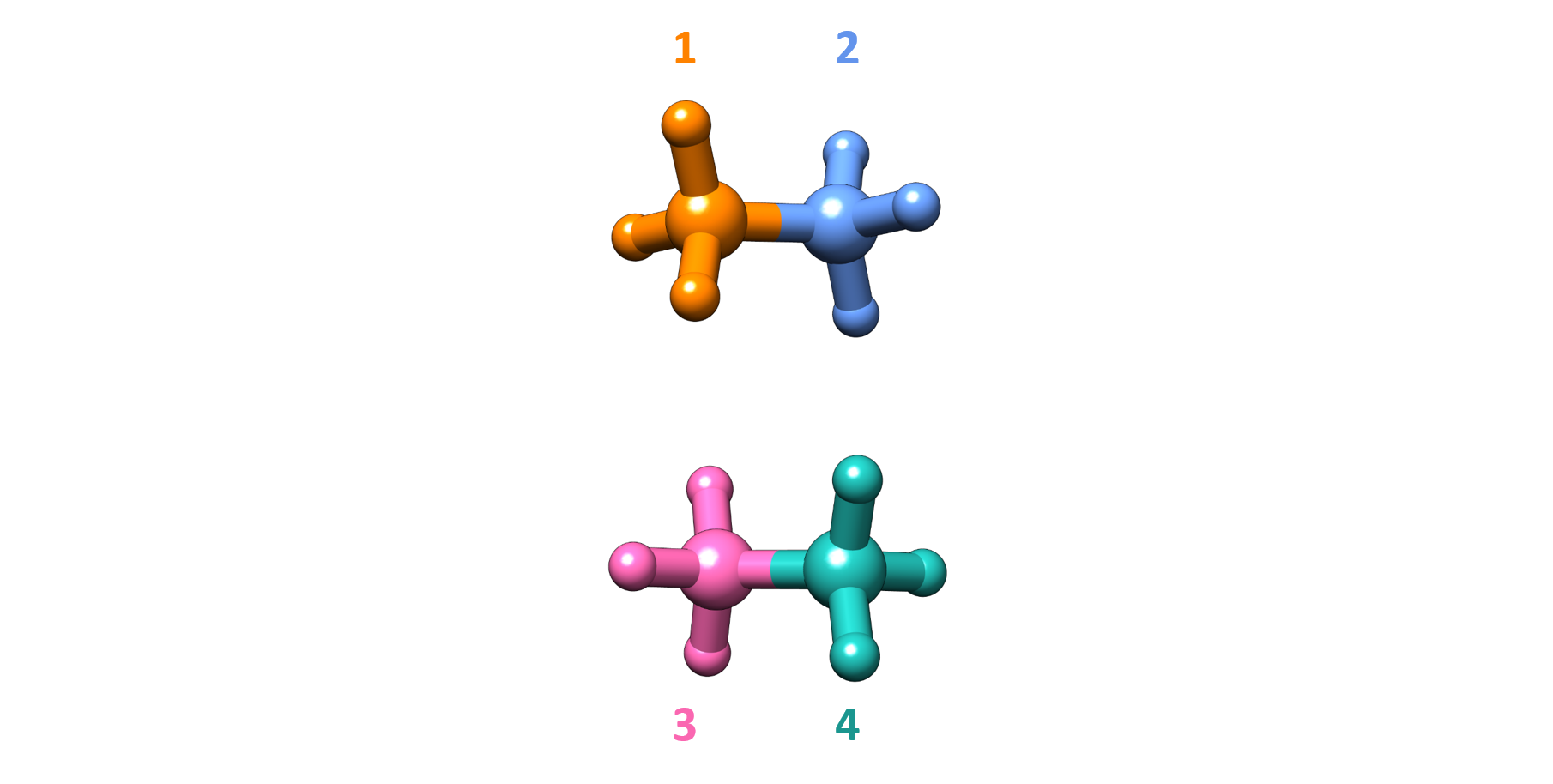
Fig. 5.71 Fragmentation scheme of the ethane dimer used in the DLPNO-CCSD(T)/COVALED calculation.
In the output file, information about the population of shared orbitals is printed out as follows:
SUMMARY ORBITALS TREATED AS COVALENT:
ORBITAL:   7; POP ATOM   4:  0.500; POP ATOM   0:  0.500
ORBITAL:  14; POP ATOM  12:  0.500; POP ATOM   8:  0.500
Then, the decomposition of the total energy into intra- and inter-fragment terms is printed. The output structure is the same as that of the standard LED approach (see Section Section 5.36.2), with the main difference lying in the values of the intra- and inter-fragment terms. Unlike the standard LED method, which assigns all the shared electron density to a single fragment, with the COVALED approach the electron density is assigned based on the population analysis of the shared orbitals, thus providing a chemically meaningful decomposition of the total energy.
As with standard LED, COVALED can be used to decompose intermolecular interaction energy into fragment-based contributions. For the ethane dimer considered above, the interaction energy is computed as the difference between the energy of the dimer and that of the two isolated ethane molecules, with geometries fixed to those in the dimer. The resulting interaction energy decomposition from both standard LED and COVALED is shown as heat maps in Fig. 5.72, where the diagonal elements represent the intra-fragment (electronic preparation) energy terms and the off-diagonal elements correspond to the interaction energy between fragment pairs.
 a) LED map
 b) COVALED map
Fig. 5.72 Heat map representation of the decomposed interaction energy between two ethane molecule within the standard LED (a) and COVALED (b) schemes, plotted using the LEDAW software [793].
Note that the total interaction energy remains unchanged, but the way it is distributed among the fragments differs between the standard LED and the COVALED approach.
Important
For a more chemically intuitive analysis of interaction energy terms, the [fp-LED](see Section {numref} sec:spectroscopyproperties.led.multifrag_led) scheme can also be
applied to the standard LED and COVALED results.
5.36.5.3. Keywords
Keyword |
Description |
|---|---|
|
Activates LED scheme |
Keyword |
Options |
Description |
|---|---|---|
|
|
Defines the indexes of atoms connected through a covalent bond. Is defined automatically if |
|
|
If true, the shared electron density is equally partitioned between the two fragments (by default, it is set to true). |
5.36.6. Dispersion Interaction Density plot
The Dispersion Interaction Density (DID) plot provides a simple yet powerful tool for the spatial analysis of the London dispersion
interaction between a pair of fragments extracted from the LED analysis in the DLPNO-CCSD(T) framework [786].
A similar scheme was developed for the closed shell local MP2 method [794]. The “dispersion energy density”,
which is necessary for generating the DID plot, can be obtained from a simple LED calculation by adding DoDIDplot true in the %mdci block.
!DLPNO-CCSD(T) ... LED
%mdci DoDIDplot true end
These can be converted to a format readable by standard visualization
programs, e.g. a cube file, through orca_plot. To do that, call
orca_plot with the command:
orca_plot gbwfilename -i
and follow the instructions that will appear on your screen, i.e.:
1 - Enter type of plot
2 - Enter no of orbital to plot
3 - Enter operator of orbital (0=alpha,1=beta)
4 - Enter number of grid intervals
5 - Select output file format
6 - Plot CIS/TD-DFT difference densities
7 - Plot CIS/TD-DFT transition densities
8 - Set AO(=1) vs MO(=0) to plot
9 - List all available densities

10 - Generate the plot
11 - exit this program
Type “1” for selecting the plot type. A few options are possible:
1 -   molecular orbitals
2 -   (scf) electron density      ......  (scfp  )  - available
3 -   (scf) spin density          ......  (scfr  )  - available
4 -   natural orbitals
5 -   corresponding orbitals
6 -   atomic orbitals
7 -   mdci electron density       ......  (mdcip )  - NOT available
8 -   mdci spin density           ......  (mdcir )  - NOT available
9 -   OO-RI-MP2 density           ......  (pmp2re)  - NOT available
10 -   OO-RI-MP2 spin density      ......  (pmp2ur)  - NOT available
11 -   MP2 relaxed density         ......  (pmp2re)  - NOT available
12 -   MP2 unrelaxed density       ......  (pmp2ur)  - NOT available
13 -   MP2 relaxed spin density    ......  (rmp2re)  - NOT available
14 -   MP2 unrelaxed spin density  ......  (rmp2ur)  - NOT available
15 -   LED dispersion interaction density  (ded21 )  - available
16 -   Atom pair density
17 -   Shielding Tensors
18 -   Polarisability Tensor
Select “LED dispersion interaction density” from the list by typing “15”. Afterwards, choose your favorite format and generate the file.
5.36.7. Automatic Fragmentation
ORCA can automatically define the fragments for the LED analysis. By default, the program will attempt to identify all monomers in the system that are not connected by covalent bonds and assign a fragment to each. However, users can define alternative fragmentation procedures, as explained in the Automatic Fragmentation section.
The XYZ coordinates of the fragments are reported in the beginning of the output file. For instance, given the input:
! dlpno-ccsd(t) cc-pvdz cc-pvdz/c cc-pvtz/jk rijk verytightscf TightPNO LED

*xyz 0 1
C    0.18726407287156      0.08210467619149      0.19811955853244
H    1.07120465088431     -0.00229078749404     -0.46002874025040
H   -0.15524644515923      1.12171178448874      0.04316776563623
O   -1.47509614629583     -1.29358571885374      2.29818864036820
H   -0.87783948760158     -0.98540169212890      1.58987042714267
H   -1.22399221548771     -2.20523304094991      2.47014489963764
*
The program will automatically identify the H\(_2\)O and the CH\(_2\) fragments.
----------------------------------------------
CARTESIAN COORDINATES OF FRAGMENTS (ANGSTROEM)
----------------------------------------------

 FRAGMENT 1
  C     0.187264    0.082105    0.198120
  H     1.071205   -0.002291   -0.460029
  H    -0.155246    1.121712    0.043168

 FRAGMENT 2
  O    -1.475096   -1.293586    2.298189
  H    -0.877839   -0.985402    1.589870
  H    -1.223992   -2.205233    2.470145
Note that this procedure works for an arbitrary number of interacting molecules. It is also possible to assign only certain atoms to a fragment and let the program define the other ones:
! dlpno-ccsd(t) cc-pvdz cc-pvdz/c cc-pvtz/jk rijk verytightscf TightPNO LED

*xyz 0 1
C(1)    0.18726407287156      0.08210467619149      0.19811955853244
H(1)    1.07120465088431     -0.00229078749404     -0.46002874025040
H(1)   -0.15524644515923      1.12171178448874      0.04316776563623
O   -1.47509614629583     -1.29358571885374      2.29818864036820
H   -0.87783948760158     -0.98540169212890      1.58987042714267
H   -1.22399221548771     -2.20523304094991      2.47014489963764
*
Important
If any atom is left unassigned (or explicitly assigned to fragment 0), it will be automatically assigned to a fragment using the Automatic Fragmentation. In such cases, the highest manually assigned fragment number must be less than the total number of fragments generated by the combination of manual and automatic procedures. If this condition is not met, ORCA will automatically reorder all fragment numbers in ascending order, starting from 1.
5.36.8. Additional Features, Defaults and List of Keywords
Note
Starting from ORCA 4.2 the default localization scheme for the PNOs has changed from PM (Pipek Mezey) to FB (Foster Boys). This might cause slight numerical differences in the LED terms with respect to that obtained from previous ORCA versions. To obtain results that are fully consistent with previous ORCA versions, PM must be specified (see below).
The following options can be used in accordance with LED.
! DLPNO-CCSD(T) cc-pVDZ cc-pVDZ/C cc-pVTZ/JK RIJK TightPNO LED TightSCF

%mdci
  LED 1               # localization method for the PNOs. Choices:
                      # 1 = PipekMezey
                      # 2 = FosterBoys (default starting from ORCA 4.2)
  PrintLevel 3        # Selects large output for LED and prints the
                      # detailed contribution
                      # of each DLPNO-CCSD strong pair
  LocMaxIterLed 600   # Maximum number of localization iterations for PNOs
  LocTolLed     1e-6  # Absolute threshold for the localization procedure for PNOs
  Maxiter 0           # Skips the CCSD iterations and
                      # the decomposition of the correlation energy
  DoLEDHF true        # Decomposes the reference energy in the LED part.
                      # By default, it is set to true.
end
Note
Starting from ORCA 4.2 an RIJCOSX implementation of the LED scheme for the decomposition of the reference energy is also available. This is extremely efficient for large systems. For consistency, the RIJCOSX variant of the LED is used only if the underlying SCF treatment is performed using the RIJCOSX approximation, i.e., if RIJCOSX is specified in the simple input line. An example of input follows.
!  dlpno-ccsd(t) def2-TZVP def2-TZVP/C def2/j rijcosx verytightscf TightPNO LED

*xyz 0 1
C(1)    0.18726407287156      0.08210467619149      0.19811955853244
H(1)    1.07120465088431     -0.00229078749404     -0.46002874025040
H(1)   -0.15524644515923      1.12171178448874      0.04316776563623
O(2)   -1.47509614629583     -1.29358571885374      2.29818864036820
H(2)   -0.87783948760158     -0.98540169212890      1.58987042714267
H(2)   -1.22399221548771     -2.20523304094991      2.47014489963764
*
Finally, here are some tips for advanced users.
The LED scheme can be used in conjunction with an arbitrary number of fragments.
The LED scheme can be used to decompose DLPNO-CCSD and DLPNO-CCSD(T) energies. At the moment, it is not possible to use this scheme to decompose DLPNO-MP2 energies directly. However, for closed shell systems, one can obtain DLPNO-MP2 energies from a DLPNO-CCSD calculation by adding a series of keywords in the
%mdciblock: (i)TScalePairsMP2PreScr 0; (ii)UseFullLMP2Guess true; (iii)TCutPairs 10(or any large value). The LED can be used as usual to decompose the resulting energy.For a closed shell system of two fragments (say A and B), the LED scheme can be used to further decompose the LED components of the reference HF energy (intrafragment, electrostatics and exchange) into a sum of frozen state and orbital relaxation correction contributions. More information can be found in Ref. [786].
To obtain the frozen state terms one has to: (i) generate a
.gbwfile containing the orbitals of both fragments (AB.gbw) usingorca_mergefrag A.gbw B.gbw AB.gbw, whereA.gbwandB.gbware the orbital files of isolated fragments at the adduct geometry; (ii) run the LED as usual by usingMOReadto read the orbitals in theAB.gbwfile in conjunction withMaxiter 0in both the%scfblock (to skip the SCF iterations) and the%mdciblock (to skip the unnecessary CCSD iterations).
Keyword |
Description |
|---|---|
|
Activates the Local Energy Decomposition |
Keyword |
Options |
Description |
|---|---|---|
|
|
PipekMezey used as localization method for the PNOs |
|
FosterBoys used as localization method for the PNOs (default starting from ORCA 4.2) |
|
|
|
Selects large output for LED and prints the detailed contribution of each DLPNO-CCSD strong pair |
|
|
Maximum number of localization iterations for PNOs (set to 600 by default) |
|
|
Absolute threshold for the localization procedure for PNOs (set to 1e-6 by default) |
|
|
Skips the CCSD iterations and the decomposition of the correlation energy |
|
|
Decomposes the reference energy in the LED part (set to true by default) |
5.36.9. Atomic Decomposition Methods
Starting from ORCA 6.1, within the LED framework, it is possible to quantify the interfragment atomic contributions to London dispersion [774](ADLD. The decomposition of DFT-D London dispersion energies is described in Section 5.38) and exchange energies (ADEX):
These atomic decomposition methods are available for both closed- and open-shell DLPNO-based methods (e.g., HFLD, DLPNO-CCSD, DLPNO-CCSD(T)). Different charge partition schemes (Mulliken and Löwdin) are available for the decomposition analysis, with Löwdin set as the default. For each scheme, the analysis reports the corresponding energy for each atom and fragment in the system, with values expressed in atomic units.
Different charge-partitioning schemes can be enabled or disabled by setting the corresponding keyword to true/false in the %mdci block:
AD_Mullikenfor Mulliken-based decompositionAD_Loewdinfor Löwdin-based decomposition
Note
The results are inherently dependent on the chosen molecular fragment definition.
If the contributions from triple excitations are included in the calculation of the LED-based method, ADLD will print the integrated contributions accordingly.
By enabling the AD_SpinResolved flag within the %mdci block, the calculation will include spin-resolved atomic contributions
for open-shell systems. This means that the energy contributions will be explicitly computed for each spin-spin interaction
separately: alpha-alpha (↑↑), beta-beta (↓↓), and alpha-beta (↑↓).
Note
Please note that contributions from triple excitations are not yet implemented in the spin-resolved decomposition.
5.36.9.1. Atomic Decomposition of London Dispersion Energy (ADLD(LED))
In systems held together by non-covalent interactions, the dominant correlation contribution to the interaction energy is LD [795]. Therefore, a first estimate of the atomic contribution to the interaction energy, computed using a post-HF scheme, can be obtained by decomposing the correlation contribution to the binding energy into atomic components [796]:
Since \(\epsilon_A\) incorporates both the long-range and the short-range dynamic correlation energy, “pure” dispersion energy at the atomic level can be isolated at the Local Energy Decomposition level:
5.36.9.1.1. Basic Usage
The atomic decomposition of dispersion energy is invoked using the !ADLD keyword.
! DLPNO-CCSD def2-TZVP def2-TZVP/C def2/JK LED ADLD
Important
Make sure to also include the !LED keyword in the simple input line
5.36.9.1.2. Example
As an example, the input file to compute the dispersion interaction between two water molecule at the DLPNO-CCSD(T)/LED level using def2-TZVP basis set along with matching /JK and /C auxiliary basis sets is reported below.
! DLPNO-CCSD(T) def2-TZVP def2-TZVP/C def2/JK LED ADLD

%mdci
	AD_Mulliken  true
	AD_Loewdin   true
end

# H2O dimer geometry optimized at B3LYP-D4/def2-TZVP level.

* xyz 0 1
  O(1)       0.00736774224494      0.01160693915772      0.01654049355157
  H(1)       0.96923953706804      0.01163512314627     -0.00786387302697
  H(1)      -0.23645852051665      0.94172445362186     -0.01797690491825
  O(2)      -0.98965374142797     -1.29474095640989      2.41552530001642
  H(2)      -0.69837507632022     -0.90508483715064      1.57804074703869
  H(2)      -1.52582551183659     -2.04783550111168      2.15519678840530
*
The corresponding output file is reported below.
-------------------------------------------------------------------------
              ADLD - Atomic Decomposition of London Dispersion
-------------------------------------------------------------------------

MULLIKEN-BASED
---------------------------------------

            ---------------------------       ---------------------------
                        CCSD                             CCSD(T)
            ---------------------------       ---------------------------

            Correlation      Dispersion       Correlation      Dispersion

1    O       -0.2187971      -0.0006293        -0.2245728      -0.0006459
2    H       -0.0215016      -0.0000253        -0.0220589      -0.0000260
3    H       -0.0214954      -0.0000249        -0.0220526      -0.0000256
4    O       -0.2183144      -0.0005019        -0.2240292      -0.0005151
5    H       -0.0205997      -0.0001578        -0.0211439      -0.0001619
6    H       -0.0225718      -0.0000199        -0.0231578      -0.0000204

Sum  =       -0.5232800      -0.0013591        -0.5370151      -0.0013949

FRAG 1       -0.2617941      -0.0006796        -0.2686843      -0.0006975
FRAG 2       -0.2614859      -0.0006796        -0.2683308      -0.0006974


LOEWDIN-BASED
---------------------------------------

            ---------------------------       ---------------------------
                        CCSD                             CCSD(T)
            ---------------------------       ---------------------------

            Correlation      Dispersion       Correlation      Dispersion

1    O       -0.2145399      -0.0006243        -0.2202052      -0.0006408
2    H       -0.0236273      -0.0000279        -0.0242397      -0.0000286
3    H       -0.0236269      -0.0000274        -0.0242394      -0.0000281
4    O       -0.2146356      -0.0004835        -0.2202539      -0.0004961
5    H       -0.0228437      -0.0001750        -0.0234472      -0.0001796
6    H       -0.0240065      -0.0000211        -0.0246297      -0.0000217

Sum  =       -0.5232800      -0.0013591        -0.5370151      -0.0013949

FRAG 1       -0.2617941      -0.0006796        -0.2686843      -0.0006975
FRAG 2       -0.2614859      -0.0006796        -0.2683308      -0.0006974
5.36.9.2. Atomic Decomposition of Exchange (ADEX(LED))
The role of interatomic exchange contributions can be studied by the atomic decomposition of exchange (ADEX) within the LED framework.
5.36.9.2.1. Basic Usage
The atomic decomposition of exchange energy is invoked using the !ADEX keyword in the simple input line.
! DLPNO-CCSD def2-TZVP def2-TZVP/C def2/JK LED ADEX
Note
ADEX is currently not available with the RIJCOSX approximation.
Important
Make sure to also include the !LED keyword in the simple input line
5.36.9.2.2. Example
As an example, the input file to compute the exchange energy between two water molecules at DLPNO-CCSD/LED level using def2-TZVP basis set along with matching /JK and /C auxiliary basis sets is reported below.
! DLPNO-CCSD def2-TZVP def2-TZVP/C def2/JK LED ADEX

%mdci
	AD_Mulliken  true
	AD_Loewdin   true
end

# H2O dimer geometry optimized at B3LYP-D4/def2-TZVP level.

* xyz 0 1
  O(1)       0.00736774224494      0.01160693915772      0.01654049355157
  H(1)       0.96923953706804      0.01163512314627     -0.00786387302697
  H(1)      -0.23645852051665      0.94172445362186     -0.01797690491825
  O(2)      -0.98965374142797     -1.29474095640989      2.41552530001642
  H(2)      -0.69837507632022     -0.90508483715064      1.57804074703869
  H(2)      -1.52582551183659     -2.04783550111168      2.15519678840530
*
The corresponding output file is reported below.
-------------------------------------------------------------------------
                 ADEX - Atomic Decomposition of Exchange
-------------------------------------------------------------------------

MULLIKEN-BASED
---------------------------------------

              Exchange

1    O       -0.0028909
2    H       -0.0000526
3    H       -0.0000536
4    O       -0.0022290
5    H       -0.0007038
6    H       -0.0000643

Sum  =       -0.0059942

FRAG 1       -0.0029971
FRAG 2       -0.0029971


LOEWDIN-BASED
---------------------------------------

              Exchange

1    O       -0.0028804
2    H       -0.0000578
3    H       -0.0000589
4    O       -0.0021483
5    H       -0.0007804
6    H       -0.0000684

Sum  =       -0.0059942

FRAG 1       -0.0029971
FRAG 2       -0.0029971
5.36.9.3. Keywords
Keyword |
Description |
|---|---|
|
Activates atomic decomposition of exchange energy |
|
Activates atomic decomposition of dispersion energy |
Keyword |
Options |
Description |
|---|---|---|
|
|
Activate Mulliken-based decomposition |
|
|
Activate Löwdin-based decomposition (default) |
|
|
Activate spin-resolved decomposition (for open-shell) |