4.1. Geometry Optimizations

ORCA is able to calculate equilibrium structures (minima and transition states) using the quasi Newton update procedure with the well known BFGS update [531, 532, 533, 534, 535, 536], the Powell or the Bofill update. The optimization can be carried out in either redundant internal (recommended in most cases) or Cartesian displacement coordinates. As initial Hessian the user can choose between a diagonal initial Hessian, several model Hessians (Swart, Lindh, Almloef, Schlegel), an exact Hessian and a partially exact Hessian (both recommended for transition state optimization) for both coordinate types. In redundant internal coordinates several options for the type of step to be taken exist. The user can define constraints via two different paths. He can either define them directly (as bond length, angle, dihedral or Cartesian constraints) or he can define several fragments and constrain the fragments internally and with respect to other fragments. The ORCA optimizer can be used as an external optimizer, i.e.the energy and gradient calculations done by ORCA.

The usage of analytic gradients is necessary for efficient geometry optimization. In ORCA 5.0, the following methods provide analytic first derivatives

• Hartree-Fock (HF) and DFT (including the RI, RIJK and RIJCOSX approximations)

• MP2, RI-MP2 and DLPNO-MP2

• TD-DFT for excited states

• CAS-SCF

When the analytic gradients are not available, it is possible to evaluate the first derivatives numerically by finite displacements. This is available for all methods.

Some methods for locating transition states (TS) require second derivative matrices (Hessian), implemented analytically for HF, DFT and MP2. Additionally, several approaches to construct an initial approximate Hessian for TS optimization are available. A very useful feature for locating complicated TSs is the Nudged-Elastic Band method in combination with the TS finding algorithm (NEB-TS, ZOOM-NEB-TS). An essential feature for chemical processes involving excited states is the conical intersection optimizer. Another interesting feature are MECP (Minimum Energy Crossing Point) optimizations.

For very large systems ORCA provides a very efficient L-BFGS optimizer, which makes use of the orca_md module. It can also be invoked via simple keywords described at the end of this section.

4.1.1. Geometry Optimizations

The use of the geometry optimization module is relatively straightforward.[1] Here are some typical examples:

! BLYP SVP Opt
* int 0 1
    C  0 0 0 0.0000   0.000    0.00
    O  1 0 0 1.2029   0.000    0.00
    H  1 2 0 1.1075 122.016    0.00
    H  1 2 3 1.1075 122.016  180.00
*

ORCA employs the RIJ by default. If this is not wanted, RI can be deactivated generally by using the !NORI keyword.

An optimization of the first excited state of ethylene:

! BLYP SVP OPT

%tddft
   IRoot 1  
end
  
* xyz 0 1
 C     0.000000     0.000000     0.666723
 C     0.000000     0.000000    -0.666723
 H     0.000000    -0.928802     1.141480
 H    -0.804366    -0.464401    -1.341480
 H     0.000000     0.928802     1.241480
 H     0.804366     0.464401    -1.241480
*

4.1.2. Initial Hessian for Minimization

The convergence of a geometry optimization crucially depends on the quality of the initial Hessian. In the simplest case it is taken as a unit matrix (in redundant internal coordinates we use 0.5 for bonds, 0.2 for angles and 0.1 for dihedrals and improper torsions). However, simple model force-fields like the ones proposed by Schlegel, Lindh, Swart or Almlöf are available and lead to much better convergence. The different guess Hessians can be set via the InHess option which can be either unit, Almloef, Lindh, Swart or Schlegel in redundant internal coordinates, furhter shown in the keywords list found within Section Geometry Optimization Keywords. Since version 2.5.30, these model force-fields (built up in internal coordinates) can also be used in optimizations in Cartesian coordinates.

For minimizations we recommend the Almloef Hessian, which is the default for minimizations. The Lindh and Schlegel Hessian yield a similar convergence behaviour. There is also the option for the Swart model Hessian, which is less parametrized and should improve for weakly interacting and/or unusual structures. Of course the best Hessian is the exact one. Read may be used to input an exact Hessian or one that has been calculated at a lower level of theory (or a “faster” level of theory). From version 2.5.30 on this option is also available in redundant internal coordinates. But we have to point out that the use of the exact Hessian as initial one is only of little help, since in these cases the convergence is usually only slightly faster, while at the same time much more time is spent in the calculation of the initial Hessian.

To sum it up: we advise to use one of the simple model force-fields for minimizations.

4.1.3. Coordinate Systems for Optimizations

The coordinate system for the optimization can be chosen by the coordsys variable that can be set to cartesian or redundantwithin the %geom block. The default is the redundant internal coordinate system. If the optimization with redundant fails, you can still try cartesian. If the optimization is then carried out in Cartesian displacement coordinates with a simple model force-field Hessian, the convergence will be only slightly slower. With a unit matrix initial Hessian very slow convergence will result.

A compound job two_step_opt.inp that first computes a semi-empirical Hessian to start from is shown below:

* int 0 1
C 0 0 0 0 0 0
O 1 0 0 1.3 0 0
H 1 2 0 1.1 110 0
H 1 2 3 1.1 110 180
*

%compound
# Step 1: semiempirical calculation of the Hessian
New_Step
! AM1 NumFreq
Step_End

# Step 2: optimization starting from previous Hessian
New_Step
!B3LYP def2-svp def2/J Opt
%geom
InHess
 Read
InHessName "two_step_opt_Compound_1.hess"
# this file must be either a .hess file from a
# frequency run or, a .opt/.carthess file left over from a
# previous geometry optimization
end
Step_End

End

Tip

• For transition metal complexes MNDO, AM1 or PM3 Hessians are not available. You can use ZINDO/1 or NDDO/1 Hessians instead. They are of lower quality than MNDO, AM1 or PM3 for organic molecules but they are still far better than the standard unit matrix choice.

• If the quality of the initial semi-empirical Hessian is not sufficient you may use a “quick” RI-DFT job (e.g. BP def2-sv(p) defgrid1)

• In semi-empirical geometry optimizations on larger molecules or in general when the molecules become larger the redundant internal space may become large and the relaxation step may take a significant fraction of the total computing time.

For condensed molecular systems and folded molecules (e.g. a U-shaped carbon chain) atoms can get very close in space, while they are distant in terms of number of bonds connecting them. As damping of optimization steps in internal coordinates might not work well for these cases, convergence can slow down. ORCA’s automatic internal coordinate generation takes care of this problem by assigning bonds to atom pairs that are close in real space, but distant in terms of number of bonds connecting them. See keywords AddExtraBonds, AddExtraBonds_MaxLength, and AddExtraBonds_MaxDist within the keyword list found in Section Geometry Optimization Keywords.

For solid systems modeled as embedded solids the automatically generated set of internal coordinates might become very large, rendering the computing time spent in the optimization routine unnecessarily large. Usually, in such calculations the cartesian positions of outer atoms, coreless ECPs and point charges are constrained during the optimization - thus most of their internal coordinates are not needed. By requesting ReduceRedInts true within the %geom block only the required needed internal coordinates (of the constrained atoms) are generated.

OBS: If the step in redundant fails badly and only Cartesian constrains are set (or no constrains), ORCA will fallback to a cartesian step automatically. This can be turned off by setting CARTFALLBACK to FALSE.

4.1.3.1. Redundant Internal Coordinates

There are three types of internal coordinates: redundant internals, old redundant internals (redundant_old) and a new set of redundant internals (redundant_new, with improved internals for nonbonded systems). All three sets work with the same “primitive” space of internal coordinates (stretches, bends, dihedral angles and improper torsions). Only the redundant internals works with one more type of bends in cases where a normal bend would have been approximately 180\(^{\circ}\). In redundant internal coordinates the full primitive set is kept and the Hessian and gradient are transformed into this – potentially large – space. A geometry optimization step requires, depending on the method used for the geometry update, perhaps a diagonalization or inversion of the Hessian of dimension equal to the number of variables in the optimization. In redundant internal coordinates this space may be 2-4 times larger than the nonredundant subspace which is of dimension 3\(N_{\mathrm{atoms} }-6(5)\). Since the diagonalization or inversion scales cubically the computational overhead over nonredundant spaces may easily reach a factor of 8–64. Thus, in redundant internal coordinates there are many unnecessary steps which may take some real time if the number of primitive internals is greater than 2000 or so (which is not so unusual). The timing problem may become acute in semiempirical calculations where the energy and gradient evaluations are cheap.

We briefly outline the theoretical background which is not difficult to understand:

Suppose, we have a set of \(n_{I}\) (redundant) primitive internal coordinates \(\mathrm{\mathbf{q} }\) constructed by some recipe and a set of \(n_{C} =3N_{\mathrm{atoms} }\) Cartesian coordinates \(\mathrm{\mathbf{x} }\). The B-matrix is defined as:

(4.1)\[B_{ij} =\frac{\partial q_{i} }{\partial x_{j} } \]

This matrix is rectangular. In order to compute the internal gradient one needs to compute the “generalized inverse” of \(\mathrm{\mathbf{B} }\). However, since the set of primitive internals is redundant the matrix is rank-deficient and one has to be careful. In practice one first computes the \(n_{I} \times n_{I}\) matrix \(\mathrm{\mathbf{G} }\):

(4.2)\[\mathrm{\mathbf{G} } = \mathrm{\mathbf{BB} }^{T} \]

The generalized inverse of \(\mathrm{\mathbf{G} }\) is denoted \(\mathrm{\mathbf{G} }^{-}\) and is defined in terms of the eigenvalues and eigenvectors of \(\mathrm{\mathbf{G} }\):

(4.3)\[\begin{split}\mathrm{\mathbf{G} }^{-}= \begin{pmatrix} \mathbf{U} \\ \mathbf{R} \end{pmatrix}^{T} \begin{pmatrix} \mathbf{\Lambda^{-1} } & \mathbf{0} \\ \mathbf{0} & \mathbf{0} \end{pmatrix} \begin{pmatrix} \mathbf{U}\\ \mathbf{R} \end{pmatrix} \end{split}\]

Here \(\mathrm{\mathbf{U} }\) are the eigenvectors belonging to the nonzero eigenvalues \(\mathrm{\mathbf{\Lambda} }\) which span the nonredundant space and \(\mathrm{\mathbf{R} }\) are the eigenvectors of the redundant subspace of the primitive internal space. If the set of primitive internals is carefully chosen, then there are exactly 3\(N_{\mathrm{atoms} }-6(5)\) nonzero eigenvalues of \(\mathrm{\mathbf{G} }\). Using this matrix, the gradient in internal coordinates can be readily computed from the (known) Cartesian gradient:

(4.4)\[\mathrm{\mathbf{g} }_{q} =\mathrm{\mathbf{G} }^{-} \mathrm{\mathbf{Bg} }_{x} \]

The initial Hessian is formed directly in the redundant internal space and then itself or its inverse is updated during the geometry optimization.

Before generating the Newton step we have to ensure that the displacements take place only in the nonredundant part of the internal coordinate space. For this purpose a projector \({P}'\):

(4.5)\[\mathbf{{P}'=GG^{-}=G^{-}G} \]

is applied on both the gradient and the Hessian:

(4.6)\[\mathbf{\tilde{g}_{q} = { P}'g_{q} } \]

(4.7)\[\mathbf{\tilde{H}_{q} = { P}'H_{q} { P}'}+\alpha \left({ \mathbf{1-{P}'} } \right)\]

The second term for \(\tilde{{H} }\) sets the matrix elements of the redundant part of the internal coordinate space to very large values (\(\alpha =1000)\).

4.1.3.2. Coordinate steps

A Quasi-Newton (QN) step is the simplest choice to update the coordinates and is given by:

(4.8)\[\mathbf{\Delta q = -\tilde{H}_{q}^{-1}\tilde{g}_{q} } \]

A more sophisticated step is the rational function optimization step which proceeds by diagonalizing the augmented Hessian:

(4.9)\[\begin{split}\begin{pmatrix} \mathbf{H}_{q} & \mathbf{g}_{q}\\ \mathbf{g}_{q} & 0 \end{pmatrix} \begin{pmatrix} \Delta \mathbf{q} \\ 1 \end{pmatrix} = v \begin{pmatrix} \Delta \mathbf{q} \\ 1 \end{pmatrix} \end{split}\]

The lowest eigenvalue \(\nu_{0}\) approaches zero as the equilibrium geometry is approached and the nice side effect of the optimization is a step size control. Towards convergence, the RFO step is approaching the quasi-Newton step and before it leads to a damped step is taken. In any case, each individual element of \(\Delta \mathrm{\mathbf{q} }\) is restricted to magnitude MaxStep and the total length of the step is restricted to Trust. In the RFO case, this is achieved by minimizing the predicted energy on the hypersphere of radius Trust which also modifies the direction of the step while in the quasi-Newton step, the step vector is simply scaled down.

Thus, the new geometry is given by:

(4.10)\[\mathrm{\mathbf{q} }_{\text{new} } =\mathrm{\mathbf{q} }_{\text{old} } +\Delta \mathrm{\mathbf{q} } \]

However, which Cartesian coordinates belong to the new redundant internal set? This is a somewhat complicated problem since the relation between internals and Cartesians is very nonlinear and the step in internal coordinates is not infinitesimal. Thus, an iterative procedure is taken to update the Cartesian coordinates. First of all consider the first (linear) step:

(4.11)\[\Delta \mathrm{\mathbf{x} }=\mathrm{\mathbf{A} }\Delta \mathrm{\mathbf{q} } \]

with \(\mathrm{\mathbf{A} }=\mathrm{\mathbf{B} }^{T}\mathrm{\mathbf{G} }^{-}\). With the new Cartesian coordinates \(\mathrm{\mathbf{x} }_{k+1} =\mathrm{\mathbf{x} }_{k} +\Delta \mathrm{\mathbf{x} }\) a trial set of internals \(\mathrm{\mathbf{q} }_{k+1}\) can be computed. This new set should ideally coincide with \(\mathrm{\mathbf{q} }_{\text{new} }\) but in fact it usually will not. Thus, one can refine the Cartesian step by forming

(4.12)\[\Delta \Delta \mathrm{\mathbf{q} }=\mathrm{\mathbf{q} }_{\text{new} } -\mathrm{\mathbf{q} }_{k+1} \]

which should approach zero. This leads to a new set of Cartesians \(\Delta \mathrm{\mathbf{x}'}=\mathrm{\mathbf{A} }\Delta \Delta \mathrm{\mathbf{q} }\) which in turn leads to a new set of internals and the procedure is iterated until the Cartesians do not change and the output internals equal \(\mathrm{\mathbf{q} }_{new}\) within a given tolerance (10\(^{-7}\) RMS deviation in both quantities is imposed in ORCA).

4.1.3.3. Constrained Optimization

Constraints on the redundant internal coordinates can be imposed by modifying the above projector \({P}'\) with a projector for the constraints \(C\):

(4.13)\[\mathbf{P}=\mathbf{{P}'-{P}'C}\left({ \mathbf{CPC} } \right)^{\mathbf{-1} }\mathbf{C{P}'} \]

\(C\) is a diagonal matrix with 1’s for the constraints and 0’s elsewhere. The gradient and the Hessian are projected with the modified projector:

(4.14)\[\tilde{{g} }_{q} =Pg_{q} \]

(4.15)\[\tilde{{H} }_{q} =PH_{q} P+\alpha \left({ 1-P} \right)\]

4.1.3.3.1. Running Constrained Optimizations - examples

You can perform constrained optimizations which can, at times, be extremely helpful. This works as shown in the following example:

! RKS B3LYP/G SV(P) Opt
%geom Constraints
        { B 0 1 1.25 C }
        { A 2 0 3 120.0 C }
        end
      end

* int 0 1
    C  0 0 0 0.0000   0.000    0.00
    O  1 0 0 1.2500   0.000    0.00
    H  1 2 0 1.1075 122.016    0.00
    H  1 2 3 1.1075 122.016  180.00
*

Constraining bond distances        :   { B N1 N2 value C }
Constraining bond angles           :   { A N1 N2 N1 value C }
Constraining dihedral angles       :   { D N1 N2 N3 N4 value C }
Constraining cartesian coordinates :   { C N1 C }
Constraining only X-coordinates    :   { X N1 C }
Constraining only Y-coordinates    :   { Y N1 C }
Constraining only Z-coordinates    :   { Z N1 C }

Note

• Like for normal optimizations you can use numerical gradients (see Numerical Gradients.) for constrained optimizations. In this case the numerical gradient will be evaluated only for non-constrained coordinates, saving a lot of computational effort, if a large part of the structure is constrained.

• “value” in the constraint input is optional. If you do not give a value, the present value in the structure is constrained. For cartesian constraints you can’t give a value, but always the initial position is constrained.

• It is recommended to use a value not too far away from your initial structure.

• It is possible to constrain whole sets of coordinates:

all bond lengths where N1 is involved       : { B N1 * C}
all bond lengths                            : { B * * C}
all bond angles where N2 is the central atom: { A * N2 * C }
all bond angles                             : { A * * * C }
all dihedral angles with central bond N2-N3 : { D * N2 N3 * C }
all dihedral angles                         : { D * * * * C }

• For Cartesian constraints (full or X/Y/Z-only) lists of atoms can be defined:

a list of atoms (10 to 17) with Cartesian constraints  : { C 10:17 C}
a list of atoms (0 to 5) with Cartesian Y constraints  : { Y 0:5 C}

• If there are only a few coordinates that have to be optimized you can use the invertConstraints option:

%geom Constraints
        { B 0 1 C }
        end
      invertConstraints true # only the C-O distance is optimized
                             # does not affect Cartesian coordinates
      end

• In some cases it is advantageous to optimize only the positions of the hydrogen atoms and let the remaining molecule skeleton fixed:

%geom optimizehydrogens true
      end

Note

• In the special case of a fragment optimization (see next point) the optimizehydrogens keyword does not fix the heteroatoms, but ensures that all hydrogen positions are relaxed.

• In Cartesian optimization, only Cartesian constraints are allowed.

4.1.3.4. Constrained Fragments and Molecular Cluster Optimization

The constrained fragments option was implemented in order to provide a convenient way to handle constraints for systems consisting of several molecules. The difference to a common optimization lies in the coordinate setup. In a common coordinate setup the internal coordinates are built up as described in the following:

In a first step, bonds are constructed between atom pairs which fulfill certain (atom type specific) distance criteria. If there are fragments in the system, which are not connected to each other (this is the case when there are two or more separate molecules), an additional bond is assigned to the nearest atom pair between the nonbonded fragments. All other internal coordinates are constructed on the basis of this set of bonds. Here, in a second step, bond angles are constructed between the atoms of directly neighboured bonds. If such an angle reaches more than 175\(^{\circ}\), a special type of linear angles is constructed. In a third step, dihedral angles (and improper torsions) are constructed between the atoms of directly neighbouring angles.

If the constrained fragments option is switched on, the set of bonds is constructed in a different way. The user defines a number of fragments (details on fragments definition can be found in Fragment Specification section.

For each fragment a full set of bonds (not seeing the atoms of the other fragments) is constructed as described above. When using this option, the user also has to define which fragments are to be connected. The connection between these fragments can either be user-defined or automatically chosen. If the user defines the connecting atoms N1 and N2, then the interfragmental bond is the one between N1 and N2. If the user does not define the interfragmental bond, it is constructed between the atom pair with nearest distance between the two fragments. Then the angles and dihedrals are constructed upon this (different) set of bonds in the already described fashion.

Now let us regard the definition of the fragment constraints: A fragment is constrained internally by constraining all internal coordinates that contain only atoms of the respective fragment. The connection between two fragments A and B is constrained by constraining specific internal coordinates that contain atoms of both fragments. For bonds, one atom has to belong to fragment A and the other atom has to belong to fragment B. Regarding angles, two atoms have to belong to fragment A and one to fragment B and vice versa. With respect to dihedrals, only those are constrained where two atoms belong to fragment A and the other two belong to fragment B.

Here is an example : if you want to study systems, which consist of several molecules (e.g. the active site of a protein) with constraints, then you can either use cartesian constraints (see above) or use ORCA’s fragment constraint option. ORCA allows the user to define fragments in the system. For each fragment one can then choose separately whether it should be optimized or constrained. Furthermore, it is possible to choose fragment pairs whose distance and orientation with respect to each other should be constrained. Here, the user can either define the atoms which make up the connection between the fragments, or the program chooses the atom pair automatically via a closest distance criterion. ORCA then chooses the respective constrained coordinates automatically. An example for this procedure is shown below.

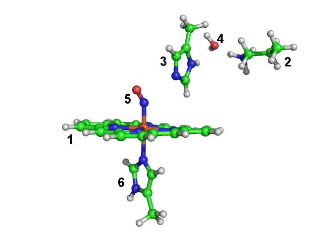
The coordinates are taken from a crystal structure [PDB-code 2FRJ]. In our gas phase model we choose only a small part of the protein, which is important for its spectroscopic properties. Our selection consists of a heme-group (fragment 1), important residues around the reaction site (lysine (fragment 2) and histidine (fragment 3)), an important water molecule (fragment 4), the NO-ligand (fragment 5) and part of a histidine (fragment 6) coordinated to the heme-iron. In this constrained optimization we want to maintain the position of the heteroatoms of the heme group. Since the protein backbone is missing, we have to constrain the orientation of lysine and histidine (fragments 2 and 3) side chains to the heme group. All other fragments (the ones which are directly bound to the heme-iron and the water molecule) are fully optimized internally and with respect to the other fragments. Since the crystal structure does not reliably resolve the hydrogen positions, we relax also the hydrogen positions of the heme group.

# !! If you want to run this optimization: be aware 
# !!  that it will take some time!
! BP86 SV(P) Opt
%geom
    ConstrainFragments { 1 } end # constrain all internal
                                 # coordinates of fragment 1
    ConnectFragments
     {1 2 C 12 28}  # connect the fragments via the atom pair 12/28 and 15/28 and
     {1 3 C 15 28}  #  constrain the internal coordinates connecting
                    #  fragments 1/2 and 1/3
      {1 5 O}
      {1 6 O}
      {2 4 O}
      {3 4 O}
    end
    optimizeHydrogens true  # do not constrain any hydrogen position
  end
* xyz 1 2
Fe(1)     -0.847213     -1.548312     -1.216237 newgto "TZVP" end
 N(5)     -0.712253     -2.291076      0.352054 newgto "TZVP" end
 O(5)     -0.521243     -3.342329      0.855804 newgto "TZVP" end
 N(6)     -0.953604     -0.686422     -3.215231 newgto "TZVP" end
 N(3)     -0.338154     -0.678533      3.030265 newgto "TZVP" end
 N(3)     -0.868050      0.768738      4.605152 newgto "TZVP" end
 N(6)     -1.770675      0.099480     -5.112455 newgto "TZVP" end
 N(1)     -2.216029     -0.133298     -0.614782 newgto "TZVP" end
 N(1)     -2.371465     -2.775999     -1.706931 newgto "TZVP" end
 N(1)      0.489683     -2.865714     -1.944343 newgto "TZVP" end
 N(1)      0.690468     -0.243375     -0.860813 newgto "TZVP" end
 N(2)      1.284320      3.558259      6.254287
 C(2)      5.049207      2.620412      6.377683
 C(2)      3.776069      3.471320      6.499073
 C(2)      2.526618      2.691959      6.084652
 C(3)     -0.599599     -0.564699      6.760567
 C(3)     -0.526122     -0.400630      5.274274
 C(3)     -0.194880     -1.277967      4.253789
 C(3)     -0.746348      0.566081      3.234394
 C(6)      0.292699      0.510431     -6.539061
 C(6)     -0.388964      0.079551     -5.279555
 C(6)      0.092848     -0.416283     -4.078708
 C(6)     -2.067764     -0.368729     -3.863111
 C(1)     -0.663232      1.693332     -0.100834
 C(1)     -4.293109     -1.414165     -0.956846
 C(1)     -1.066190     -4.647587     -2.644424
 C(1)      2.597468     -1.667470     -1.451465
 C(1)     -1.953033      1.169088     -0.235289
 C(1)     -3.187993      1.886468      0.015415
 C(1)     -4.209406      0.988964     -0.187584
 C(1)     -3.589675     -0.259849     -0.590758
 C(1)     -3.721903     -2.580894     -1.476315
 C(1)     -4.480120     -3.742821     -1.900939
 C(1)     -3.573258     -4.645939     -2.395341
 C(1)     -2.264047     -4.035699     -2.263491
 C(1)      0.211734     -4.103525     -2.488426
 C(1)      1.439292     -4.787113     -2.850669
 C(1)      2.470808     -3.954284     -2.499593
 C(1)      1.869913     -2.761303     -1.932055
 C(1)      2.037681     -0.489452     -0.943105
 C(1)      2.779195      0.652885     -0.459645
 C(1)      1.856237      1.597800     -0.084165
 C(1)      0.535175      1.024425     -0.348298
 O(4)     -1.208602      2.657534      6.962748
 H(3)     -0.347830     -1.611062      7.033565
 H(3)     -1.627274     -0.387020      7.166806
 H(3)      0.121698      0.079621      7.324626
 H(3)      0.134234     -2.323398      4.336203
 H(3)     -1.286646      1.590976      5.066768
 H(3)     -0.990234      1.312025      2.466155
 H(4)     -2.043444      3.171674      7.047572
 H(2)      1.364935      4.120133      7.126900
 H(2)      0.354760      3.035674      6.348933
 H(2)      1.194590      4.240746      5.475280
 H(2)      2.545448      2.356268      5.027434
 H(2)      2.371622      1.797317      6.723020
 H(2)      3.874443      4.385720      5.867972
 H(2)      3.657837      3.815973      7.554224
 H(2)      5.217429      2.283681      5.331496
 H(2)      5.001815      1.718797      7.026903
 H(6)     -3.086380     -0.461543     -3.469767
 H(6)     -2.456569      0.406212     -5.813597
 H(6)      1.132150     -0.595619     -3.782287
 H(6)      0.040799      1.559730     -6.816417
 H(6)      0.026444     -0.139572     -7.404408
 H(6)      1.392925      0.454387     -6.407850
 H(1)      2.033677      2.608809      0.310182
 H(1)      3.875944      0.716790     -0.424466
 H(1)      3.695978     -1.736841     -1.485681
 H(1)      3.551716     -4.118236     -2.608239
 H(1)      1.487995     -5.784645     -3.308145
 H(1)     -1.133703     -5.654603     -3.084826
 H(1)     -3.758074     -5.644867     -2.813441
 H(1)     -5.572112     -3.838210     -1.826943
 H(1)     -0.580615      2.741869      0.231737
 H(1)     -3.255623      2.942818      0.312508
 H(1)     -5.292444      1.151326     -0.096157
 H(1)     -5.390011     -1.391441     -0.858996
 H(4)     -1.370815      1.780473      7.384747
 H(2)      5.936602      3.211249      6.686961
*

Note

• You have to connect the fragments in such a way that the whole system is connected.

• You can divide a molecule into several fragments.

• Since the initial Hessian for the optimization is based upon the internal coordinates: Connect the fragments in a way that their real interaction is reflected.

• This option can be combined with the definition of constraints, scan coordinates(see Surface Scans) and the optimizeHydrogens option (but: its meaning in this context is different to its meaning in a normal optimization run, relatively straightforward see section Geometry Optimizations).

• Can be helpful in the location of complicated transition states (with relaxed surface scans), see Surface Scans.

• Since constraints must be defined manually, Automatic Fragmentation will not be enabled automatically if there are unassigned atoms to fragments. However, it can be activated by including a %frag block.

4.1.4. Optimization Assuming a Rigid Body

If you want to optimize one or multiple fragments assuming these as a “rigid bodies”, i.e. only allowing for movements of the center of mass and pure rotations for each fragment, the keyword !RIGIDBODYOPT can be used.

It needs to be combined with one of the optimization flags, such as !OPT RIGIDBODYOPT or !L-OPT RIGIDBODYOPT, and all fragments which were defined in any way will be treated as such.

For a more fine control, whenever fragments are defined for the system, each fragment can be optimized differently (similar to the fragment optimization described above). The following options are available: FixFrags,RelaxHFrags,RelaxFrags, and RigidFrags shown within Section Geometry Optimization Keywords.

A more complex example is depicted in the following:

! L-Opt # or !COPT or !OPT

*xyzfile 0 1 geometry.xyz

%frag
 Definition
  1 {0:12} end
  2 {13:17} end
  3 {18:38} end
  4 {39:53} end
 end
end

%geom
 RelaxFrags {1} end     # Fragment 1 is fully relaxed
 RigidFrags {2 3 4} end # Fragments 2, 3 and 4 are treated as rigid bodies each.
end

Note

The manual definition of fragments have to be done after the coordinate input.

Important

• If there are atoms not assigned to any fragment, Automatic Fragmentation will be enabled by default. Users can explicitly control this behavior, as described in Fragment Specification.

• Fragment enumeration will be reordered if manual assignments exceed the total number of fragments and Automatic Fragmentation is enabled. However, the values of RelaxFrags and RigidFrags will not be updated accordingly.

4.1.5. Adding Arbitrary Bias and Wall Potentials

For some applications, it might be interesting to add arbitrary bias potentials during the geometry optimization. For example, if you want to optimize an intermolecular complex and need that both structures stick together, without one flying away during the optimization, you might want to add a wall bias. Or you might need a bond bias to guide the DOCKER to dock structures onto certain specific regions of others.

Note

All these walls and biases are integrated with the other electronic-structure methods in ORCA, including their Hessian.

4.1.5.1. Bond Bias Potentials

From ORCA 6.1, we introduced a bond bias potential that can be added between two arbitrary atoms. It will effectively create a fictitious bond between atoms A and B, using a symmetric Morse-like potential:

\[\begin{aligned} V = E_{AB}(1-e^{-\alpha(R_{AB}-R_{min}})^2)\end{aligned}\]

where \(E_{AB}\) is the energy difference from the bottom of the well to the top, \(R_{min}\) is the equilibrium distance. \(\alpha\) is a decay parameter that will be automatically determined if not given such as to ensure 50% intensity at \(2 \times R_{min}\). In practice, it looks like this:

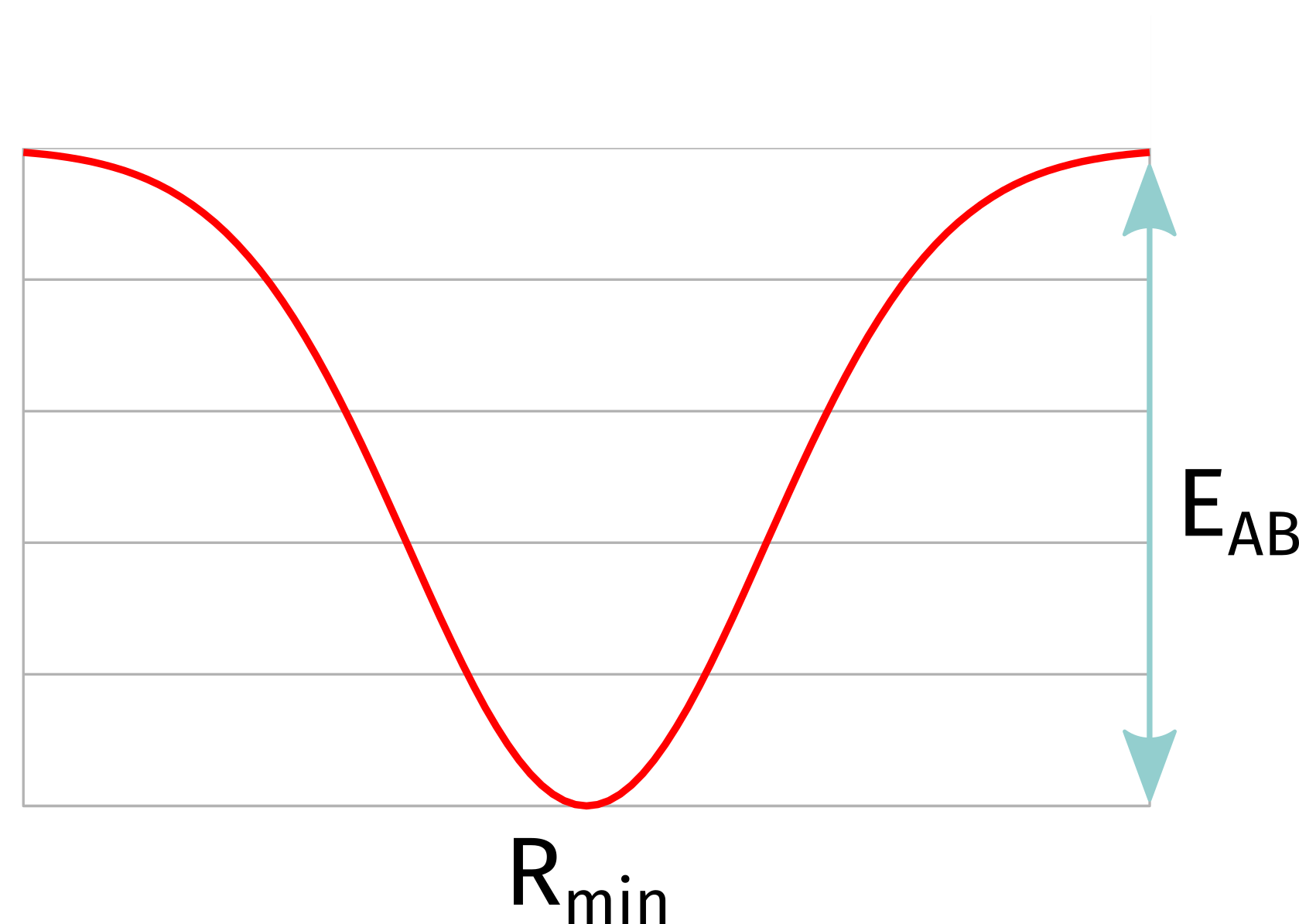
The input to create a simple bias between atoms 0 and 1 is:

%GEOM 
  BIAS { B 0 1 } END 
END

Up to three other parameters can be given: \(R_{min}\) in Angstroem, \(E_{AB}\) in kcal/mol and the alpha. If none of those are given the default values are: sum of Van der Walls radii, 25 kcal/mol and \(\alpha\) will be chosen as described above.

In order to define a bond with \(R_{min}=1.5 \mathring{A}\) and a \(E_{AB}=100kcal/mol\), for example:

%GEOM 
  BIAS { B 0 1 1.5 100 } END 
END

If a star symbol (*) is used for any of those three, that quantity will be taken from the defaults. For example, in order to set the energy depth, but not the distance, simply use:

%GEOM 
  BIAS { B 0 1 * 100 } END 
END

Note

A negative number on the \(E_{AB}\) will create the inverse, repulsive potential instead!

Important

The ORCA DOCKER has its own BIAS block and needs a different input than this to work there, please check Section Adding a bond bias to the docking process for more details.

4.1.5.2. Wall Bias Potentials

you can also add three kinds of arbitrary “wall potentials”: an ellipsoid or spherical of the form

\[\begin{aligned} V = \left(\frac{|\mathbf{R} - \mathbf{O}|}{ radius}\right)^{30}\end{aligned}\]

or a rectangular box potential with 6 walls of the form

\[\begin{aligned} V = e^{5(\mathbf{R}-wall) }\end{aligned}\]

These can be given in two ways: by explicitly defining the origin of the potential and its limits, e.g:

%GEOM 
    ELLIPSEPOT 0,0,0,5,3,4 # the last are the a,b and c radii
END

or:

%GEOM 
    SPHEREPOT 0,0,0,5 # the last is the radius
END

or:

%GEOM 
    BOXPOT 0,0,0,4,-4,3,-3,6,-6 # maxx, minx, maxy, miny, maxz and minz last
END

where the first three numbers are the center and the last is the radius for the sphere (or a,b and c for the ellipsoid) and the max and min x,y and z dimensions of the box. All numbers should be given in Ångström.

In case a single number is given instead, the walls will be automatically centered around the centroid of the molecule and that number will be added to the minimum sphere or box that is necessary to contain the molecule. For example:

%GEOM 
    SPHEREPOT 2
END

or:

%GEOM 
    BOXPOT 2
END

will build a minimum wall centered on the centroid that encloses the molecule and add 2 Ångström on top of it. Still on the sphere case, a negative number like

%GEOM 
    SPHEREPOT -2
END

will make the total radius of the sphere to be Ångström.

Note

This will apply to regular geometry optimizations, as well as to the Global Optimizer (GOAT), NEB, DOCKER, SOLVATOR, etc.

4.1.6. Constant External Force - Mechanochemistry

Constant external force can be applied on the molecule within the EFEI formalism[537] by pulling on the two defined atoms. To apply the external force, use the POTENTIALS in the geom block. The potential type is C for Constant force, indexes of two atoms (zero-based) and the value of force in nN.

! def2-svp  OPT 
%geom
  POTENTIALS
    { C 2 3 4.0 }
  end
end

 * xyz 0 1
O          0.73020       -0.07940       -0.00000
O         -0.73020        0.07940       -0.00000
H          1.21670        0.75630        0.00000
H         -1.21670       -0.75630        0.00000
 *

The results are seen in the output of the SCF procedure, where the total energy already contains the force term.

----------------
TOTAL SCF ENERGY
----------------

Total Energy       :         -150.89704913 Eh           -4106.11746 eV

Components:
Nuclear Repulsion  :           36.90074715 Eh            1004.12038 eV
External potential :           -0.25613618 Eh              -6.96982 eV
Electronic Energy  :         -187.54166010 Eh           -5103.26802 eV
:language: orca

4.1.7. Printing Hessian in Internal Coordinates

When a Hessian is available, it can be printed out in redundant internal coordinates as in the following example:

! opt
%geom inhess read
      inhessname "h2o.hess"
      PrintInternalHess true
end
*xyz 0 1
  O      0.000000    0.000000    0.000000
  H      0.968700    0.000000    0.000000
  H     -0.233013    0.940258    0.000000
*

Note

• The Hessian in internal coordinates is (for the input printHess.inp) stored in the file printHess_internal.hess.

• The corresponding lists of redundant internals is stored in printHess.opt.

• Although the !Opt keyword is necessary, an optimization is not carried out. ORCA exits after storing the Hessian in internal coordinates.

4.1.8. Using model Hessian from previous calculations

If you had a geometry optimization interrupted, or for some reason want to use the model Hessian updated from a previous calculation, you can do that by passing a basename.opt file, a basename.carthess file or the initial Hessian on a new calculation.

%GEOM 
    InHess     READ
    InHessName "basename.carthess"
END

4.1.9. Geometry Optimizations using the L-BFGS optimizer

Optimizations using the L-BFGS optimizer are done in Cartesian coordinates. They can be invoked quite simple as in the following example:

! L-Opt
! MM
%MM
  ORCAFFFILENAME "CHMH.ORCAFF.prms"
END
*pdbfile 0 1 CHMH.pdb

Using this optimizer systems with 100s of thousands of atoms can be optimized. Of course, the energy and gradient calculations should not become the bottleneck for such calculations, thus MM or QM/MM methods should be used for such large systems.

The default maximum number of iterations is 200, and can be increased as follows:

! L-Opt
%GEOM
  maxIter 500 # default 200
END
*pdbfile 0 1 CHMH.pdb

Only the hydrogen positions can be optimized with the following command:

! L-OptH

But also other elements can be exclusively optimized with the following command:

! L-OptH
%GEOM
 OptElement F  # optimize fluorine only when L-OptH is invoked.
               # Does not work with optimization in internal coordinates.
END

Note

If you want to use the previously (ORCA5 and ORCA6.0) available L-Opt option, you need to specify MD-L-Opt or MD-L-OptH.

4.1.10. Optimizing with External Methods

Although ORCA features a many electronic structure models, it cannot cover all available methods. Therefore, ORCA features an interface to external programs that allows you to use ORCA’s features with electronic structure methods and model potentials provided by external programs. This way, you’ll be able to utilize the latest MNDO based semi-empirical methods like PM7 or neural network potentials like AIMNet2 and UMA within the ORCA infrastructure, e.g. to optimize structures, search transition states with NEB-TS, or sample conformers with GOAT.

The external optimization infrastructure can be accessed via the ORCA simple input keyword !ExtOpt which can be combined with other common keywords like !Opt or !GOAT. As every program typically provides differently formatted output, individual wrapper scripts are required to link ORCA and its external optimizer infrastructure. The full path to your wrapper script can be provided via the %method block in the ORCA input file:

! ExtOpt

%method
  ProgExt "/full/path/to/wrapperscript"
  Ext_Params "optional command line arguments"
end

Alternatively, you can also provide the script as a file or link named otool_external in the same directory as the ORCA executables, or by assigning the EXTOPTEXE environment variable to the full path to the external program.

Regardless of which option is used, the keyword Ext_Params can be used to specify the additional command line arguments as a single string.

Note

All information that you give on the electronic structure is discarded.

After executing ORCA, it automatically writes an input file called basename_EXT.extinp.tmp in each step containing the following info:

basename_EXT.xyz # xyz filename: string, ending in '.xyz'
0 # charge: integer
1 # multiplicity: positive integer
1 # NCores: positive integer
0 # do gradient: 0 or 1
pointcharges.pc # point charge filename: string (optional)

Comments from # until the end of the line should be ignored. The file basename_EXT.xyz will also be written to the working directory. While the energy is always requested, the gradient is only calculated when needed.

ORCA then calls:

scriptname basename_EXT.extinp.tmp [args]

Here, args are the optional command line arguments provided defined with the Ext_Params in the ORCA input. They are passed to the external program without any changes.

The external script starts the energy (and gradient) calculation and finally provides the results in a file called basename_EXT.engrad using the same basename as the XYZ file. This file must have the following format:

#
# Number of atoms: must match the XYZ
#
3
#
# The current total energy in Eh
#
-5.504066223730
#
# The current gradient in Eh/bohr: Atom1X, Atom1Y, Atom1Z, Atom2X, etc.
#
-0.000123241583
0.000000000160
-0.000000000160
0.000215247283
-0.000000001861
0.000000001861
-0.000092005700
0.000000001701
-0.000000001701

Comments from # until the end of the line are ignored, as are any comment-only lines.

The script may also print relevant output to STDOUT and/or STDERR. STDOUT will either be printed in the ORCA standard output, or redirected to a temporary file and removed afterwards, depending on the type of job (e.g., for NumFreq the output for the displaced geometries is always redirected) and the ORCA output settings:

%output
  Print[P_EXT_OUT]  1 # (default) print the external program output
  Print[P_EXT_GRAD] 1 # (default) print the gradient from the ext. program
end

Important

Some wrapper scripts and how to use them can be found in the official GitHub repository. While some methods and programs such as MOPAC, AIMNet2, and UMA are already supported, you are free to write your own wrapper scripts to extend the available methods usable with ORCA. If you do so, please contribute to the repository via pull requests to share with the community.

Note

Note that depending on your OS and infrastructure, you may need to do some modifications to the wrapper script.

4.1.11. Optimization FAQs

4.1.11.1. I can’t locate the transition state (TS) for a reaction expected to feature a low/very low barrier, what should I do?

For such critical case of locating the TS, running a very fine (e.g. 0.01 Å increment of the bond length) relaxed scan of the key reaction coordinate is recommended, see Surface Scans. In this way the highest energy point on a very shallow surface can be identified and used for the final TS optimisation.

4.1.11.2. During the geometry optimisation some atoms merge into each other and the optimisation fails. How can this problem be solved?

This usually occurs due to the wrong or poor construction of initial molecular orbital involving some atoms. Check the basis set definition on problematic atoms and then the corresponding MOs!

4.1.12. Geometry Optimization Keywords

Table 4.1 Simple input keywords for geometry optimization.

Keyword	Description
Opt	Optimization with default convergence tolerance (Alias: NormalOpt)
LooseOpt	Optimization with looser convergence tolerance
TightOpt	Optimization with tight convergence tolerance
VeryTightOpt	Optimization with very tight convergence tolerance
COpt	Optimization in Cartesian coordinates (can be combined with TightOpt, etc.)

Table 4.2 %method block input keywords and options for geometry optimization.

Keyword	Option / Value	Description
%method	RunTyp Opt	Sets geometry optimization as the run type.
	RunTyp=Geom	Alternative syntax for geometry optimization.

Table 4.3 %geom block input keywords and options for geometry optimization.

Keyword	Option / Value	Description
MaxIter	50	Maximum number of geometry iterations (default max(3N, 50)).
coordsys	redundant	Use redundant internal coordinates.
	cartesian	Use Cartesian coordinates.
cartfallback	true	Use Cartesian step if internal coordinate step fails.
modify_internal	{B 10 0 A}	Add bond between atoms 0 and 10.
	{A 8 9 10 R}	Remove angle between atoms 8, 9, and 10.
	{D 7 8 9 10 R}	Remove dihedral between atoms 7, 8, 9, and 10.
Constraints	{B 1 2 value C}	Constrain bond between atoms 1 and N.
	{A 1 2 3 value C}	Constrain angle defined by atoms 1, 2, and 3.
	{D 1 2 3 4 value C}	Constrain dihedral defined by atoms 1–4.
	{C 1 C}	Constrain Cartesian position of atom 1.
	{B 1 * C}	Constrain all bonds involving atom 1.
	{B * * C}	Constrain all bonds.
	{A * 2 * C}	Constrain all angles with atom 2 as central.
	{A * * * C}	Constrain all angles.
	{D * 2 3 * C}	Constrain all dihedrals with 2 and 3 as central atoms.
	{D * * * * C}	Constrain all dihedrals.
ReduceRedInts	true	Generates the internal coordinates of the constrains atoms.
ConnectFragments	{1 3 O}	Optimize internal coordinates connecting fragments 1 and 3.
	{1 3 O N1 N2}	Connect fragments 1 and 3 via atoms N1 and N2.
ConstrainFragments	{1}	Constrain all internal coordinates within fragment 1.
Frags	X {0:12}	Defining fragment X, containing atoms 0-12. Note that all other atoms not specified in the Frags keyword belong to fragment 1 by default.
AUTOFRAG	true	Automatically select fragments based on topology
FixFrags	{1}	Freeze the coordinates of all atoms of the specified fragment(s).
RelaxHFrags	{1}	Relax the hydrogen atoms of the specified fragment(s). Default for all atoms if !L-OptH is defined.
RelaxFrags	{1}	Relax all atoms of the specified fragment(s). Default for all atoms if !L-Opt is defined.
RigidFrags	{1}	Treat each specified fragment as a rigid body, but relax the position and orientation of these rigid bodies.
optimizeHydrogens	true	Optimize coordinates involving H atoms while constraining others.
freezeHydrogens	true	Freeze H positions relative to heteroatoms.
invertConstraints	true	Invert the defined constraints (only affects redundant internals).
Step	qn	Use quasi-Newton step.
	rfo	Use Rational Function Optimization step (default for !Opt).
	prfo	Use partitioned RFO step (default for !OptTS).
MaxStep	0.3	Maximum step length in internal coordinates (default: 0.3 au).
Trust	-0.3	Use fixed trust radius of 0.3 au (negative sign indicates fixed).
TolE	5e-6	Convergence threshold for energy change (a.u.).
TolRMSG	1e-4	Convergence threshold for RMS gradient (a.u.).
TolMaxG	3e-4	Convergence threshold for max gradient component (a.u.).
TolRMSD	2e-3	Convergence threshold for RMS displacement (a.u.).
TolMaxD	4e-3	Convergence threshold for max displacement (a.u.).
Convergence	normal	Default convergence threshold.
	loose	Looser convergence thresholds.
	tight	Tighter convergence thresholds.
ProjectTR	false	Disable translation and rotation projection (must be false for internals).
inhess	unit	Start optimization with a unit matrix Hessian.
	Read	Read Hessian from external file. Requires InHessName.
InHessName	"filename.hess"	Specifies file containing the Hessian (e.g., .hess, .opt, .carthess).
	Lindh	Use Lindh’s model Hessian (only for redundant coordinates).
	Almloef	Use Almloef’s model Hessian.
	Schlegel	Use Schlegel’s model Hessian.
	Swart	Use Swart and Bickelhaupt’s model Hessian.
	XTB0	Use GFN0-xTB Hessian.
	XTB1	Use GFN1-xTB Hessian.
	XTB2	Use GFN2-xTB Hessian.
	GFNFF	Use GFN-FF Hessian.
Calc_Hess	true	Calculate numerical Hessian at the beginning of optimization.
Recalc_Hess	5	Recalculate Hessian every 5 cycles.
Hybrid_Hess	{0 1 5 6} end	Calculate exact Hessian for specified atoms, use model for the rest.
NumHess	true	Request numerical Hessian.
Hess_Internal	{A 3 2 1 D 2.0}	Manually set Hessian value (Eh/Bohr²) for angle between atoms 3-2-1.
	reset 5	Reset modified Hessian values after 5 cycles.
	{B 1 0 C}	Coordinates for Hessian refinement after a relaxed surface scan.
	XYZ1 "scanName.003.xyz"	Structure file before maximum in scan.
	XYZ2 "ScanName.005.xyz"	Structure file after maximum in scan.
	GBW1 "ScanName.003.gbw"	Optional GBW file before max in scan.
	GBW2 "ScanName.005.xyz"	Optional GBW file after max in scan.
Update	Powell	Use Powell update for Hessian.
	Bofill	Use Bofill update (default for TS optimization).
	BFGS	Use BFGS update (default for geometry optimization).
HESS_Modification	Shift_Diag	Shift diagonal elements of Hessian (default).
	EV_Reverse	Reverse sign of diagonal elements.
HESS_MinEV	0.0001	Minimum allowed Hessian eigenvalue.
NResetHess	20	Rebuild model Hessian after 20 steps (BFGS only).
NStepsInResetHess	5	Number of previous steps used to inform new model Hessian.
UseSOSCF	false	Switches the converger to SOSCF after the first point. May converge better than DIIS if the starting orbitals are good. Default: false.
ReducePrint	true	Reduces printout after the first point. Default: true.
OptGuess		The initial guess can be changed after the first point. The default is MORead. The MOs of the previous point will in many cases be a very good guess for the next point. In some cases however, you may want to be more conservative and use a general guess.
OptGuess	OneElec	Use the one-electron matrix guess.
	Hueckel	Use the extended Hückel guess.
	PAtom	Use the PAtom guess.
	PModel	Use the PModel guess.
	MORead	Use MOs of the previous point. Default.
AddExtraBonds	true	Enables assigning bonds to atom pairs connected by more than MaxLength bonds and less than MaxDist Å apart. Default: true.
AddExtraBonds_MaxLength	10	Maximum number of bonds connecting two atoms to consider for extra bonding. Default: 10.
AddExtraBonds_MaxDist	5	Maximum distance (in Å) between two atoms to be considered for extra bonding. Default: 5.
BIAS	{B 0 1}	Create a fictitious bond between atoms 1 and 2 to create Morse-like potential
ELLIPSEPOT	0,0,0,5,3,4	Defines an ellipsoidal potential centered at (0,0,0) with semi-axes a=5, b=3, c=4.
SPHEREPOT	0,0,0,5	Defines a spherical potential centered at (0,0,0) with radius 5.
BOXPOT	0,0,0,4,-4,3,-3,6,-6	Defines a box potential: maxx=4, minx=–4, maxy=3, miny=–3, maxz=6, minz=–6.
OptElement	N	Optimize element “N” atoms only (requires L-OptH; not compatible with internal coordinates).

---

[1]

But that doesn’t mean that geometry optimization itself is straightforward! Sometimes, even when it is not expected the convergence can be pretty bad and it may take a better starting structure to come to a stationary point. In particular floppy structures with many possible rotations around single bonds and soft dihedral angle modes are tricky. It may sometimes be advantageous to compute a Hessian matrix at a “cheap” level of theory and then do the optimization in Cartesian coordinates starting from the calculated Hessian.