3.10. Coupled Cluster and CI Theories (MDCI)
Aside from the second-order Møller-Plesset theory (MP2),
ORCA features a variety of single-reference correlation methods for
single point energies (restricted to a RHF or RKS determinant in the
closed-shell case and a UHF or UKS determinant in the open-shell case;
quasi-restricted orbitals (QROs)[356] are also supported in the
open-shell case). These methods are all fairly expensive but maybe be used in
order to obtain accurate results in the case that the reference
determinant is a good starting point for the expansion of the many-body
wavefunction. The methods are implemented in the orca_mdci module, which is the main subject of this section.
‘MDCI’ is an abbreviations for “matrix driven configuration interaction”. The term is rather
technical to emphasize that if one wants to implement these methods (CCSD, QCISD etc.)
efficiently, one needs to write them in terms of matrix operations, which
pretty much every computer can drive at peak performance.
It should be noted that in recent years, a number of highly correlated single reference methods and their properties were added to ORCA using automatic code generation and reside in the orca_autoci module,
which follows similar design principles.[357, 358] Let us first briefly describe the theoretical background of the methods, that we have
implemented in ORCA.
3.10.1. Theory
We start from the full CI hierarchy in which the wavefunction is expanded as:
where \(\left| 0 \right\rangle\) is a single-determinant reference and S, D, T, Q, …denote the single, double, triple quadruple and higher excitations relative to this determinant at the spin-orbital level. As usual, labels \(i,j,k,l\) refer to occupied orbitals in \(\left| 0 \right\rangle\), \(a,b,c,d\) to unoccupied MOs and \(p,q,r,s\) to general MOs. The action of the second quantized excitation operators \(a_{i}^{a} =a_{a}^{\dagger} a_{i}\) on \(\left| 0 \right\rangle\) lead to excited determinants \(\left| \Phi_i^a \right\rangle\) that enter \(\left| \Psi \right\rangle\) with coefficients \(C_{a}^{i}\). The variational equations are:
Further equations coupling triples with singles through pentuples etc.
The total energy is the sum of the reference energy \(E_{0} =\left\langle {0\left| H \right|0} \right\rangle\) and the correlation energy
which requires the exact singles- and doubles amplitudes to be known. In order to truncate the series to singles- and doubles one may either neglect the terms containing the higher excitations on the right hand side (leading to CISD) or approximate their effect thereby losing the variational character of the CI method (CCSD, QCISD and CEPA methods). Defining the one- and two-body excitation operators as \(\hat{{C} }_{1} =\sum\nolimits_{ia} {C_{a}^{i} a_{i}^{a} }\), \(\hat{{C} }_{2} =\frac{1}{4}\sum\nolimits_{ijab} {C_{ab}^{ij} a_{ij}^{ab} }\) one can proceed to approximate the triples and quadruples by the disconnected terms:
As is well known, the CCSD equations contain many more disconnected contributions arising from the various powers of the \(\hat{{C} }_{1}\) operator (if one would stick to CC logics one would usually label the cluster amplitudes with \(t_{a}^{i} ,t_{ab}^{ij}\),…and the \(n\)-body cluster operators with \(\hat{{T} }_{n}\); we take a CI point of view here). In order to obtain the CEPA type equations from ((3.88)-(3.92)), it is most transparent to relabel the singles and doubles excitations with a compound label \(P\) for the internal indices (\(i\)) or (ij) and \(x\) for (\(a\)) or (ab). Then, the approximations are as follows:
Here the second line contains the approximation that only the terms in which either Qy or Rz are equal to Px are kept (this destroys the unitary invariance) and the fourth line contains the approximation that only “exclusion principle violating” (EPV) terms of internal labels are considered. The notation \(Qy\cup Px\) means “Qy joint with Px” (containing common orbital indices) and \(\varepsilon_{Q}\) is the pair correlation energy. The EPV terms must be subtracted from the correlation energy since they arise from double excitations that are impossible due to the fact that an excitation out of an occupied or into an empty orbital of the reference determinant has already been performed. Inserting eq. (3.96) into eq. (3.89) \(C_{x}^{P} E_{C}\) cancels and effectively is replaced by the “partial correlation energy” \(\sum\nolimits_{Q\cup P} { \varepsilon_{Q} }\).
The resulting equations thus have the appearance of a diagonally shifted
(“dressed”) CISD equation
\(\left\langle { \Phi_{P}^{x} \left|{ H-E_{0}
+\Delta } \right|0+S+D} \right\rangle=0\). If the second approximation
mentioned above is avoided Malrieu’s (SC) \(^{2}\)-CISD arises.
[307, 308, 309, 310, 359]
Otherwise, one obtains CEPA/3 with the shift:
CEPA/2 is obtained by \(-\Delta_{ab}^{ij} =\varepsilon_{ij}\) and CEPA/1 is the average of the CEPA/2 and CEPA/3. As mentioned by Ahlrichs, [360] no consensus appears to exist in the literature for the appropriate shift on the single excitations. If one proceeds straightforwardly in the same way as above, one obtains:
as the appropriate effect of the disconnected triples on the singles. It has been assumed here that only the singles \(\left|\Phi_i^a \right\rangle\) in \(\hat{{C} }_{1}\) contribute to the shift. If \(\left| 0 \right\rangle\) is a HF determinant, the effect of the disconnected triples in the doubles projection vanishes under the same CEPA approximations owing to Brillouin’s theorem. Averaged CEPA models are derived by assuming that all pair correlation energies are equal (except \(\varepsilon_{ii} =0)\). As previously discussed by Gdanitz [361], the averaging of CEPA/1 yields \(\frac{2}{n}E_{\text{C} }\) and CEPA/3 \(E_{\text{C} } \frac{4n-6}{n\left({ n-1} \right)}\) where \(n\) is the number of correlated electrons. These happen to be the shifts used for the averaged coupled-pair functional (ACPF [362]) and averaged quadratic coupled-cluster (AQCC [363]) methods respectively. However, averaging the singles shift of eq. (3.98) gives \(\frac{4}{n}E_{\text{C} }\). The latter is also the leading term in the expansion of the AQCC shift for large \(n\). In view of the instability of ACPF in certain situations, Gdanitz has proposed to use the AQCC shift for the singles and the original ACPF shift for the doubles and called his new method ACPF/2 [362]. Based on what has been argued above, we feel that it would be most consistent with the ACPF approach to simply use \(\frac{4}{n}E_{\text{C} }\) as the appropriate singles shift. We refer to this as NACPF.
It is readily demonstrated that the averaged models may be obtained by a variation of the modified correlation energy functional:
with g\(_{S}\) and g\(_{D}\) being the statistical factors \(\frac{4}{n}\), \(\frac{2}{n}\), \(\frac{4n-6}{n\left({ n-1} \right)}\), as appropriate for the given method. Thus, unlike the CEPA models, the averaged models fulfill a stationarity principle and are unitarily invariant. However, if one thinks about localized internal MOs, it appears evident that the approximation of equal pair energies must be one of rather limited validity and that a more detailed treatment of the electron pairs is warranted. Maintaining a stationarity principle while providing a treatment of the pairs that closely resembles that of the CEPA methods was achieved by Ahlrichs and co-workers in an ingenious way with the development of the CPF method [364]. In this method, the correlation energy functional is written as:
with
The topological matrix for pairs \(P=\)(ij) and \(Q=(kl)\) is chosen as: [115]
with \(n_{i}\) being the number of electrons in orbital \(i\) in the reference determinant. The singles out of orbital \(i\) are formally equated with \(P=(ii)\). At the spin-orbital level, \(n_{i} =1\), for closed shells \(n_{i} =2\). Using the same topological matrix in \(\Delta_{P} =\sum\nolimits_Q { T_{PQ} \varepsilon_{Q} }\) one recovers the CEPA/1 shifts for the doubles in eq. (3.98). It is straightforward to obtain the CPF equivalents of the other CEPA models by adjusting the \(T_{PQ}\) matrix appropriately. In our program, we have done so and we refer below to these methods as CPF/1, CPF/2 and CPF/3 in analogy to the CEPA models (CPF/1 \(\equiv\)CPF). In fact, as discussed by Ahlrichs and co-workers, variation of the CPF-functional leads to equations that very closely resemble the CEPA equation and can be readily implemented along the same lines as a simple modification of a CISD program. Ahlrichs et al. argued that the energies of CEPA/1 and CPF/1 should be very close. We have independently confirmed that in the majority of cases, the total energies predicted by the two methods differ by less than 0.1 mEh.
An alternative to the CPF approach which is also based on variational optimization of an energy functional is the VCEPA method [365]. The equations resulting from application of the variational principle to the VCEPA functional are even closer to the CEPA equations than for CPF so that the resulting energies are practically indistinguishable from the corresponding CEPA values. The VCEPA variants are referred to as VCEPA/1, VCEPA/2, and VCEPA/3 in analogy to CEPA and CPF. A strictly size extensive energy functional (SEOI) which is invariant with respect to unitary transformations within the occupied and virtual orbital subspaces is also available [366] (an open-shell version is not implemented yet).
Again, a somewhat critical point concerns the single excitations. They do not account for a large fraction of the correlation energy. However, large coefficients of the single excitations lead to instability and deterioration of the results. Secondly, linear response properties are highly dependent on the effective energies of the singles and their balanced treatment is therefore important. Since the CEPA and CPF methods amount to shifting down the diagonal energies of the singles and doubles, instabilities are expected if the effective energy of an excitation approaches the reference energy of even falls below it. In the CPF method this would show up as denominators \(N_{P}\) that are too small. The argument that the CPF denominators are too small has led Chong and Langhoff to the proposal of the MCPF method which uses a slightly more elaborate averaging than (\(N_{P}N_{Q})^{1/2}\) [367].[1] However, their modification was solely based on numerical arguments rather than physical or mathematical reasoning. In the light of Eq. (3.98) and the performance of the NACPF, it appears to us that for the singles one should use twice the \(T_{PQ}\) proposed by Ahlrichs and co-workers. The topological matrix \(T_{PQ}\) is modified in the following way for the (very slightly) modified method to which we refer to as NCPF/1:
(note that \(T_{PQ} \ne T_{QP}\) for this choice). Thus, the effect of the singles on the doubles is set to zero based on the analysis of the CEPA approximations and the effect of the singles on the singles is also set to zero. This is a sensible choice since the product of two single excitations is a double excitation which is already included in the SD space and thus none of them can belong to the outer space. It is straightforward to adapt this reasoning about the single excitations to the CEPA versions as well as to NCPF/2 and NCPF/3.
The aforementioned ambiguities arising from the use of single excitations in coupled-pair methods can be avoided by using correlation-adapted orbitals instead of Hartree-Fock orbitals thus eliminating the single excitations. There are two alternatives: (a) Brueckner orbitals and (b) optimized orbitals obtained from the variational optimization of the electronic energy with respect to the orbitals. Both approaches have already been used for the coupled-cluster doubles (CCD) method [368, 369] and later been extended to coupled-pair methods [370]. In the case of CCD, orbital optimization requires the solution of so-called \(\Lambda\) (or Z vector) equations [371]. There is, however, a cheaper alternative approximating the Z vector by a simple analytical formula [372].
Furthermore, the parametrized coupled-cluster (pCCSD) method of
Huntington and Nooijen [373], which combines the
accuracy of coupled-pair type methods for (usually superior to CCSD, at
least for energies and energy differences) with the higher stability of
the coupled-cluster methods, is an attractive alternative. Comprehensive
numerical tests [374] indicate that particularly
pCCSD(-1,1,1) (or pCCSD/1a) and pCCSD (-1.5,1,1) (or pCCSD/2a) have
great potential for accurate computational thermochemistry. These
methods can be employed by adding the “simple” keywords pCCSD/1a or
pCCSD/2a to the first line of input. As mentioned in section
Local correlation (DLPNO), the DLPNO
variants of the pCCSD/1a method is also available for RHF and UHF
references via the simple keyword DLPNO-pCCSD/1a.
3.10.1.1. Closed-Shell Equations
Proceeding from spin-orbitals to the spatial orbitals of a closed-shell determinant leads to the actual working equations of this work. Saebo, Meyer and Pulay have exploited the generator state formalism to arrive at a set of highly efficient equations for the CISD problem [375]. A similar set of matrix formulated equations for the CCSD and QCISD cases has been discussed by Werner and co-workers [376] and the MOLPRO implementation is widely recognized to be particularly efficient. Equivalent explicit equations for the CISD and CCSD methods were published by Scuseria et al. [377][2] The doubles equations for the residual “vector” \(\mathbf{\sigma}\) are (\(i\leqslant j\), all \(a,b\)):
The singles equations are:
The following definitions apply:
The two-electron integrals are written in (11|12) notation and F is the closed-shell Fock operator with F \(^{V}\)being its virtual sub-block. We do not assume the validity of Brillouin’s theorem. The amplitudes \(C_{a}^{i} ,\,C_{ab}^{ij}\) have been collected in vectors \(\mathrm{\mathbf{C} }^{i}\) and matrices \(\mathrm{\mathbf{C} }^{ij}\) wherever appropriate. The shifts \(\Delta^{i}\) and \(\Delta^{ij}\) are dependent on the method used and are defined in Table Table 3.35 for each method implemented in ORCA.
Method |
Doubles Shift |
Singles Shift |
|---|---|---|
CISD |
\(E_{\text{C} }\) |
\(E_{\mathbf{C} }\) |
CEPA/0 |
0 |
0 |
CEPA/1 |
\(\frac{1}{2}(\varepsilon_{i} +\varepsilon_{j} )+\frac{1}{4}\sum\limits_k { (\varepsilon_{ik} +\varepsilon_{jk} ) }\) |
\(\frac{1}{2}\varepsilon_{ii} +\frac{1}{2}\sum\limits_k { \varepsilon_{ik} }\) |
CEPA/2 |
\(\delta_{ij} \varepsilon_{i} +\varepsilon_{ij}\) |
\(\varepsilon_{i} +\varepsilon_{ii}\) |
CEPA/3 |
\((\varepsilon_{i} +\varepsilon_{j} )-\delta_{ij} \varepsilon_{i} -\varepsilon_{ij} +\frac{1}{2}\sum\limits_k { (\varepsilon_{ik} +\varepsilon_{jk} ) }\) |
\(\varepsilon_{i} +\sum\limits_k { \varepsilon_{ik} }\) |
NCEPA/1 |
\(\frac{1}{4}\sum\limits_k { (\varepsilon_{ik} +\varepsilon_{jk} ) }\) |
\(\varepsilon_{ii} +\sum\limits_k { \varepsilon_{ik} }\) |
NCEPA/2 |
\(\varepsilon_{ij}\) |
\(2\varepsilon_{ii}\) |
NCEPA/3 |
\(-\varepsilon_{ij} +\frac{1}{2}\sum\limits_k { (\varepsilon_{ik} +\varepsilon_{jk} ) }\) |
\(2\sum\limits_k { \varepsilon_{ik} }\) |
CPF/1 |
\(N_{ij} \left\{{ \frac{1}{2}(\frac{\varepsilon_{i} }{N_{i} }+\frac{\varepsilon_{j} }{N_{j} })+\frac{1}{4}\sum\limits_k { (\frac{\varepsilon_{ik} }{N_{ik} }+\frac{\varepsilon_{jk} }{N_{jk} }) } } \right\}\) |
\(N_{i} \left\{{ \frac{1}{2}\frac{\varepsilon_{ii} }{N_{ii} }+\frac{1}{2}\sum\limits_k { \frac{\varepsilon_{ik} }{N_{ik} } } } \right\}\) |
CPF/2 |
\(N_{ij} \left\{{ \delta_{ij} \frac{\varepsilon_{i} }{N_{i} }+\frac{\varepsilon_{ij} }{N_{ij} } } \right\}\) |
\(N_{i} \left\{{ \frac{\varepsilon_{i} }{N_{i} }+\frac{\varepsilon_{ii} }{N_{ii} } } \right\}\) |
CPF/3 |
\(N_{ij} \left\{{ \frac{\varepsilon_{i} }{N_{i} }\left({ 1-\delta_{ij} } \right)+\frac{\varepsilon_{j} }{N_{j} }-\frac{\varepsilon_{ij} }{N_{ij} }+\frac{1}{2}\sum\limits_k { (\frac{\varepsilon_{ik} }{N_{ik} }+\frac{\varepsilon_{jk} }{N_{jk} }) } } \right\}\) |
\(N_{i} \left\{{ \frac{\varepsilon_{i} }{N_{i} }+\sum\limits_k { \frac{\varepsilon_{ik} }{N_{ik} } } } \right\}\) |
NCPF/1 |
\(\frac{1}{4}N_{ij} \sum\limits_k { (\frac{\varepsilon_{ik} }{N_{ik} }+\frac{\varepsilon_{jk} }{N_{jk} }) }\) |
\(N_{i} \left\{{ \frac{\varepsilon_{ii} }{N_{ii} }+\sum\limits_k { \frac{\varepsilon_{ik} }{N_{ik} } } } \right\}\) |
NCPF/2 |
\(N_{ij} \frac{\varepsilon_{ij} }{N_{ij} }\) |
\(2N_{i} \frac{\varepsilon_{ii} }{N_{ii} }\) |
NCPF/3 |
\(N_{ij} \left\{{ -\frac{\varepsilon_{ij} }{N_{ij} }+\frac{1}{2}\sum\limits_k { (\frac{\varepsilon_{ik} }{N_{ik} }+\frac{\varepsilon_{jk} }{N_{jk} }) } } \right\}\) |
\(2N_{i} \sum\limits_k { \frac{\varepsilon_{ik} }{N_{ik} } }\) |
ACPF |
\(\frac{2}{n}E_{\text{C} }\) |
\(\frac{2}{n}E_{\text{C} }\) |
ACPF/2 |
\(\frac{2}{n}E_{\text{C} }\) |
\(\left[{ 1-\frac{(n-3)(n-2) }{n(n-1) }} \right]E_{\text{C} }\) |
NACPF |
\(\frac{2}{n}E_{\text{C} }\) |
\(\frac{4}{n}E_{\text{C} }\) |
AQCC |
\(\left[{ 1-\frac{(n-3)(n-2) }{n(n-1) }} \right]E_{\text{C} }\) |
\(\left[{ 1-\frac{(n-3)(n-2) }{n(n-1) }} \right]E_{\text{C} }\) |
The QCISD method requires some slight modifications. We found it most convenient to think about the effect of the nonlinear terms as a “dressing” of the integrals occurring in equations (3.107) and (3.108). This attitude is close to the recent arguments of Heully and Malrieu and may even open interesting new routes towards the calculation of excited states and the incorporation of connected triple excitations.[378] The dressed integrals are given by:
The CCSD method can be written in a similar way but requires 15 additional terms that we do not document here. They may be taken conveniently from our paper about the LPNO-CCSD method [379].
A somewhat subtle point concerns the definition of the shifts in making the transition from spin-orbitals to spatial orbitals. For example, the CEPA/2 shift becomes in the generator state formalism:
(\(\tilde{{\Phi } }_{ij}^{ab}\) is a contravariant configuration state function, see Pulay et al. [371]. The parallel and antiparallel spin pair energies are given by:
This formulation would maintain the exact equivalence of an orbital and a spin-orbital based code. Only in the (unrealistic) case that the parallel and antiparallel pair correlation energies are equal the CEPA/2 shift of Table 3.35 arise. However, we have not found it possible to maintain the same equivalence for the CPF method since the electron pairs defined by the generator state formalism are a combination of parallel and antiparallel spin pairs. In order to maintain the maximum degree of internal consistency we have therefore decided to follow the proposal of Ahlrichs and co-workers and use the topological matrix \(T_{PQ}\) in equation (3.102) and the equivalents thereof in the CEPA and CPF methods that we have programmed.
3.10.1.2. Open-Shell Equations
We have used a non-redundant set of three spin cases (\(\alpha \alpha\), \(\beta \beta\), \(\alpha \beta\)) for which the doubles amplitudes are optimized separately. The equations in the spin-unrestricted formalism are straightforwardly obtained from the corresponding spin orbital equations by integrating out the spin. For implementing the unrestricted QCISD and CCSD method, we applied the same strategy (dressed integrals) as in the spin-restricted case. The resulting equations are quite cumbersome and will not be shown here explicitly [380].
Note that the definitions of the spin-unrestricted CEPA shifts differ from those of the spin-restricted formalism described above (see Kollmar et al. [380]). Therefore, except for CEPA/1 and VCEPA/1 (and of course CEPA/0), for which the spin-adaptation of the shift can be done in a consistent way, CEPA calculations of closed-shell molecules yield slightly different energies for the spin-restricted and spin-unrestricted versions. Since variant 1 is also the most accurate among the various CEPA variants [381], we recommend to use variant 1 for coupled-pair type calculations. For the variants 2 and 3, reaction energies of reactions involving closed-shell and open-shell molecules simultaneously should be calculated using the spin-unrestricted versions only.
A subtle point for open-shell correlation methods is the choice of the reference determinant [382]. Single reference correlation methods only yield reliable results if the reference determinant already provides a good description of the systems electronic structure. However, an UHF reference wavefunction suffers from spin-contamination which can spoil the results and lead to convergence problems. This can be avoided if quasi-restricted orbitals (QROs) are used [356, 378] since the corresponding zeroth-order wavefunction is an eigenfunction of the \(\hat{{S} }^{2}\) operator and thus, no severe spin-contamination will appear. The coupled-pair and coupled-cluster equations will be still solved in a spin-unrestricted formalism but the energy will be slightly higher compared to the results obtained with a spin-polarized UHF reference determinant. Furthermore, especially for more difficult systems like e.g. transition metal complexes, it is often advantageous to use Kohn-Sham (KS) orbitals instead of HF orbitals.
3.10.2. Basic Usage
The coupled-cluster and CI methods in orca_mdci are available for RHF and UHF
references. The implementation is fairly efficient and suitable for
large-scale calculations. The most elementary use of this module is
fairly simple.
!  METHOD
# where METHOD is:
#   CCSD CCSD(T) QCISD QCISD(T) CPF/n NCPF/n CEPA/n NCEPA/n
#   (n=1,2,3 for all variants) ACPF NACPF AQCC CISD

!  AOX-METHOD
# computes contributions from integrals with 3- and 4-external
# labels directly from AO integrals that are pre-stored in a
# packed format suitable for efficient processing

!  AO-METHOD
# computes contributions from integrals with 3- and 4-external
# labels directly from AO integrals. Can be done for integral
# direct and conventional runs. In particular, the conventional
# calculations can be very efficient

!  MO-METHOD   (this is the default)
# performs a full four index integral transformation. This is
# also often a good choice

!  RI-METHOD
# selects the RI approximation for all integrals. Rarely advisable

!  RI34-METHOD
# selects the RI approximation for the integrals with 3- and 4-
# external labels
#
# The module has many additional options that are documented
# later in the manual.

! RCSinglesFock
! RIJKSinglesFock
! NoRCSinglesFock
! NoRIJKSinglesFock
# Keywords to select the way the so-called singles Fock calculation
# is evaluated. The first two keywords turn on, the second two turn off
# RIJCOSX or RIJK, respectively.
Note
The same FrozenCore options as for MP2 are applied in the MDCI module.
Since ORCA 4.2, an additional term, called “4th-order doubles-triples correction” is considered in open-shell CCSD(T). To reproduce previous results, one should use a keyword,
%mdci
  Include_4thOrder_DT_in_Triples  false
end
The MDCI module cannot deal with systems without alpha virtual orbitals, even if there are beta virtual orbitals. Normally this only happens when the user uses minimal basis sets.
The computational effort for these methods is high — O(N\(^6\)) for all methods and O(N\(^7\)) if the triples correction is to be computed (calculations based on an unrestricted determinant are roughly 3 times more expensive than closed-shell calculations and approximately six times more expensive if triple excitations are to be calculated). This restricts the calculations somewhat: on presently available PCs 300–400 basis functions are feasible and if you are patient and stretch it to the limit it may be possible to go up to 500–600; if not too many electrons are correlated maybe even up to 800–900 basis functions (when using AO-direct methods).
Tip
For calculations on small molecules and large basis sets the MO-METHOD option is usually the most efficient; say perhaps up to about 300 basis functions. For integral conventional runs, the AO-METHOD may even more efficient.
For large calculations (>300 basis functions) the AO-METHOD option is a good choice. If, however, you use very deeply contracted basis sets such as ANOs these calculations should be run in the integral conventional mode.
AOX-METHOD is usually slightly less efficient than MO-METHOD or AO-METHOD.
RI-METHOD is seldom the most efficient choice. If the integral transformation time is an issue than you can select
%mdci trafotype trafo_rior choose RI-METHOD and then%mdci kcopt kc_ao.Regarding the singles Fock keywords (RCSinglesFock, etc.), the program usually decides which method to use to evaluate the singles Fock term. For more details on the nature of this term, and options related to its evaluation, see The singles Fock term.
To put this into perspective, consider a calculation on serine with the cc-pVDZ basis set — a basis on the lower end of what is suitable for a highly correlated calculation. The time required to solve the equations is listed in Table 3.36. We can draw the following conclusions:
As long as one can store the integrals and the I/O system of the computer is not the bottleneck, the most efficient way to do coupled-cluster type calculations is usually to go via the full transformation (it scales as O(N\(^5\)) whereas the later steps scale as O(N\(^6\)) and O(N\(^7\)) respectively).
AO-based coupled-cluster calculations are not much inferior. For larger basis sets (i.e. when the ratio of virtual to occupied orbitals is larger), the computation times will be even more favorable for the AO based implementation. The AO direct method uses much less disk space. However, when you use a very expensive basis set the overhead will be larger than what is observed in this example. Hence, conventionally stored integrals — if affordable — are a good choice.
AOX-based calculations run at essentially the same speed as AO-based calculations. Since AOX-based calculations take four times as much disk space, they are pretty much outdated and the AOX implementation is only kept for historical reasons.
RI-based coupled-cluster methods are significantly slower. There are some disk space savings, but the computationally dominant steps are executed less efficiently.
CCSD is at most 10% more expensive than QCISD. With the latest AO implementation the awkward coupled-cluster terms are handled efficiently.
CEPA is not much more than 20% faster than CCSD. In many cases CEPA results will be better than CCSD and then it is a real saving compared to CCSD(T), which is the most rigorous.
If triples are included practically the same comments apply for MO versus AO based implementations as in the case of CCSD.
ORCA is quite efficient in this type of calculation, but it is also clear that the range of application of these rigorous methods is limited as long as one uses canonical MOs. ORCA implements novel variants of the so-called local coupled-cluster method which can calculate large, real-life molecules in a linear scaling time. This will be addressed in Sec. Local correlation (DLPNO).
Method |
SCFMode |
Time (min) |
|---|---|---|
MO-CCSD |
|
38.2 |
AO-CCSD |
|
47.5 |
AO-CCSD |
|
50.8 |
AOX-CCSD |
|
48.7 |
RI-CCSD |
|
64.3 |
AO-QCISD |
|
44.8 |
AO-CEPA/1 |
|
40.5 |
MO-CCSD(T) |
|
147.0 |
AO-CCSD(T) |
|
156.7 |
All of these methods are designed to cover dynamic correlation in systems where the Hartree-Fock determinant dominates the wavefunctions. The least attractive of these methods is CISD which is not size-consistent and therefore practically useless. The most rigorous are CCSD(T) and QCISD(T). The former is perhaps to be preferred, since it is more stable in difficult situations.[3] One can get highly accurate results from such calculations. However, one only gets this accuracy in conjunction with large basis sets. It is perhaps not very meaningful to perform a CCSD(T) calculation with a double-zeta basis set (see Table 3.37). The very least basis set quality required for meaningful results would perhaps be something like def2-TZVP(-f) or preferably def2-TZVPP (cc-pVTZ, ano-pVTZ). For accurate results quadruple-zeta and even larger basis sets are required and at this stage the method is restricted to rather small systems.
Let us look at the case of the potential energy surface of the N\(_2\) molecule. We study it with three different basis sets: TZVP, TZVPP and QZVP. The input is the following:
! TZVPP CCSD(T)
%paras R= 1.05,1.13,8
       end
* xyz 0 1
N 0 0 0
N 0 0 {R}
*
For even higher accuracy we would need to introduce relativistic effects and - in particular - turn the core correlation on.[4]
Method |
Basis set |
\(\mathrm{R}_\mathbf{e}\) (pm) |
\(\omega_{\mathbf{e} }\) (cm\(^{\mathbf{-1} }\)) |
\(\omega_{\mathbf{e} }\) x\(_{\mathbf{e\, } }\)(cm\(^{\mathbf{-1} }\)) |
|---|---|---|---|---|
CCSD(T) |
SVP |
111.2 |
2397 |
14.4 |
TZVP |
110.5 |
2354 |
14.9 |
|
TZVPP |
110.2 |
2349 |
14.1 |
|
QZVP |
110.0 |
2357 |
14.3 |
|
ano-pVDZ |
111.3 |
2320 |
14.9 |
|
ano-pVTZ |
110.5 |
2337 |
14.4 |
|
ano-pVQZ |
110.1 |
2351 |
14.5 |
|
CCSD |
QZVP |
109.3 |
2437 |
13.5 |
Exp |
109.7 |
2358.57 |
14.32 |
One can see from Table 3.37 that for high accuracy - in particular for the vibrational frequency - one needs both - the connected triple-excitations and large basis sets (the TZVP result is fortuitously good). While this is an isolated example, the conclusion holds more generally. If one pushes it, CCSD(T) has an accuracy (for reasonably well-behaved systems) of approximately 0.2 pm in distances, <10 cm\(^{-1}\) for harmonic frequencies and a few kcal/mol for atomization energies.[5] It is also astonishing how well the Ahlrichs basis sets do in these calculations — even slightly better than the much more elaborate ANO bases.
Note
The quality of a given calculation is not always high because it carries the label “coupled-cluster”. Accurate results are only obtained in conjunction with large basis sets and for systems where the HF approximation is a good 0\(^{th}\) order starting point.
3.10.2.1. Frozen Core Options
In coupled-cluster calculations the Frozen Core (FC) approximation is applied by default. This implies that the core electrons are not included in the correlation treatment, since the inclusion of dynamic correlation in the core electrons usually affects relative energies insignificantly.
The frozen core option can be switched on or off with ! FrozenCore or
! NoFrozenCore in the simple input. More information and further
options are given in section
Frozen Core Options and in section
Including (semi)core orbitals in the correlation treatment.
3.10.2.2. The singles Fock term
In most MDCI calculations, there is an intermediate, which resembles closely to the SCF Fock matrix, and similar methods are available to efficiently calculate it. In the followings, a short discussion will be given of the so-called singles Fock term, which in the closed shell case has the form
The singles Fock matrix can be obtained via transformation from its counterpart (\(G(\mathbf{t}_1)_{\mu\nu}\)) in the atomic orbital (AO) basis
where
is the analogue of the SCF density matrix for the singles Fock case. For the singles Coulomb (\(J(\mathbf{t}_1)_{\mu\nu}\)) case, the density may be symmetrized (\(\tilde{P}(\mathbf{t}_1)_{\kappa\tau}=P(\mathbf{t}_1)_{\kappa\tau}+P(\mathbf{t}_1)_{\tau\kappa}\)), and one may use the resolution of identity approximation
where \(A, B\) are elements of the RI/DF auxiliary fitting basis. Note that the factor of 2 in ((3.122)) is taken care of by symmetrization. Since we are using a symmetric density, we may use the same efficient routine to evaluate the singles Coulomb term as in the SCF case, see RI-J and Split-RI-J.
For the exchange case (\(K(\mathbf{t}_1)_{\mu\nu}\)), one possibility is to use the COSX approximation (see RIJCOSX)
The COSX routine is able to deal with asymmetric densities as well, and thus, it can be used here similar to the SCF case.
The other possibility is to use RI for exchange (RIK),
where
and the \(\tilde{j}\) is an “orbital” transformed using \(C(\mathbf{t}_1)\).
Using these approximations, there are two approximations for the total singles Fock term, RIJCOSX called by the simple keyword RCSinglesFock and RIJK called by RIJKSinglesFock, see Basic Usage. For canonical and LPNO methods, by default the program chooses the same approximation used in the SCF calculation. DLPNO2013 uses RIJCOSX by default, while in DLPNO, the singles Fock term is also evaluated using PNOs via SinglesFockUsePNOs, see Local correlation (DLPNO). This behavior can also be changed by keywords in the method block.
%method RIJKSinglesFock 1   # 0 false, 1 true
        RCSinglesFock   0   # 0 false, 1 true
end
3.10.3. Coupled-Cluster Densities
If one is mainly accustomed to Hartree-Fock or DFT calculations, the calculation of the density matrix is more or less a triviality and is automatically done together with the solution of the self-consistent field equations. Unfortunately, this is not the case in coupled-cluster theory (and also not in MP2 theory). The underlying reason is that in coupled-cluster theory, the expansion of the exponential \(e^{\hat T}\) in the expectation value
only terminates if all possible excitation levels are exhausted, i.e., if all electrons in the reference determinant \(\Psi _0\) (typically the HF determinant) are excited from the space of occupied to the space of virtual orbitals (here \(D_{pq}^{}\) denotes the first order density matrix, \(E_p^q\) are the spin traced second quantized orbital replacement operators, and \(\hat T\) is the cluster operator). Hence, the straightforward application of these equations is far too expensive. It is, however, possible to expand the exponentials and only keep the linear term. This then defines a linearized density which coincides with the density that one would calculate from linearized coupled-cluster theory (CEPA/0). The difference to the CEPA/0 density is that converged coupled-cluster amplitudes are used for its evaluation. This density is straightforward to compute and the computational effort for the evaluation is very low. Hence, this is a density that can be easily produced in a coupled-cluster run. It is not, however, what coupled-cluster aficionados would accept as a density.
The subject of a density in coupled-cluster theory is approached from the viewpoint of response theory. Imagine one adds a perturbation of the form
to the Hamiltonian. Then it is always possible to cast the first derivative of the total energy in the form:
This is a nice result. The quantity \(D_{pq}^{\text{(response)}}\) is the so-called response density. In the case of CC theory where the energy is not obtained by variational optimization of an energy functional, the energy has to be replaced by a Lagrangian reading as follows:
Here \(\langle \Phi_\eta |\) denotes any excited determinant (singly, doubly, triply, ….). There are two sets of Lagrange multipliers: the quantities \(z_{ai}\) that guarantee that the perturbed wavefunction fulfills the Hartree-Fock conditions by making the off-diagonal Fock matrix blocks zero and the quantities \(\lambda_{\eta}\) that guarantee that the coupled-cluster projection equations for the amplitudes are fulfilled. If both sets of conditions are fulfilled then the coupled-cluster Lagrangian simply evaluates to the coupled-cluster energy. The coupled-cluster Lagrangian can be made stationary with respect to the Lagrangian multipliers \(z_{ai}\) and \(\lambda_{\eta}\). The response density is then defined through:
The density \(D_{pq}\) appearing in this equation does not have the same properties as the density that would arise from an expectation value. For example, the response density can have eigenvalues lower than 0 or larger than 2. In practice, the response density is, however, the best “density” there is for coupled-cluster theory.
Unfortunately, the calculation of the coupled-cluster response density is quite involved because additional sets of equations need to be solved in order to determine the \(z_{ai}\) and \(\lambda_{\eta}\). If only the equations for \(\lambda_{\eta}\) are solved one speaks of an “unrelaxed” coupled-cluster density. If both sets of equations are solved, one speaks of a “relaxed” coupled-cluster density. For most intents and purposes, the orbital relaxation effects incorporated into the relaxed density are small for a coupled-cluster density. This is so, because the coupled-cluster equations contain the exponential of the single excitation operator \(e^{\hat T_1} = \exp (\sum_{ai} t_a^iE_i^a)\). This brings in most of the effects of orbital relaxation. In fact, replacing the \(\hat T_1\) operator by the operator \(\hat\kappa = \sum_{ai} \kappa_a^i(E_i^a - E_a^i)\) would provide all of the orbital relaxation thus leading to “orbital optimized coupled-cluster theory” (OOCC).
Not surprisingly, the equations that determine the coefficients \(\lambda_{\eta}\) (the Lambda equations) are as complicated as the coupled-cluster amplitude equations themselves. Hence, the calculation of the unrelaxed coupled-cluster density matrix is about twice as expensive as the calculation of the coupled-cluster energy (but not quite as with proper program organization terms can be reused and the Lambda equations are linear equations that converge somewhat better than the non-linear amplitude equations).
ORCA features the calculation of the unrelaxed coupled-cluster density on the basis of the Lambda equations for closed- and open-shell systems. If a fully relaxed coupled-cluster density is desired then ORCA still features the orbital-optimized coupled-cluster doubles method (OOCCD). This is not exactly equivalent to the fully relaxed CCSD density matrix because of the operator \(\hat\kappa\) instead of \(\hat T_1\). However, results are very close and orbital optimized coupled-cluster doubles is the method of choice if orbital relaxation effects are presumed to be large.
In terms of ORCA keywords, the coupled-cluster density is obtained through the following keywords:
#
# coupled-cluster density
#
%mdci  density   none
                 linearized
                 unrelaxed
                 orbopt
       end
which will work together with CCSD or QCISD (QCISD and CCSD are identical in the case of OOCCD because of the absence of single excitations). Note, that an unrelaxed density for CCSD(T) is NOT available.
Instead of using the density option “orbopt” in the mdci-block, OOCCD can also be invoked by using the keyword:
! OOCCD
3.10.4. Static versus Dynamic Correlation
Let us look at an “abuse” of the single reference correlation methods by studying (very superficially) a system which is not well described by a single HF determinant. This already occurs for the twisting of the double bond of C\(_2\)H\(_4\). At a 90\(^{\circ}\) twist angle the system behaves like a diradical and should be described by a multireference method (see section Complete and Incomplete Active Space Self-Consistent Field (CASSCF and RAS/ORMAS))

Fig. 3.4 A rigid scan along the twisting coordinate of C\(_2\)H\(_4\). The inset shows the T\(_1\) diagnostic for the CCSD calculation.
As can be seen in Fig. 3.4, there is a steep rise in energy as one approaches a 90\(^{\circ}\) twist angle. The HF curve is actually discontinuous and has a cusp at 90\(^{\circ}\). This is immediately fixed by a simple CASSCF(2,2) calculation which gives a smooth potential energy surface. Dynamic correlation is treated on top of the CASSCF(2,2) method with the MRACPF approach as follows:
#
# twisting the double bond of C2H4
#
! SV(P) def2-TZVP/C SmallPrint NoPop MRACPF
%casscf nel         2
        norb        2
        mult        1
        nroots      1
        TrafoStep  RI
        end
%mrci   tsel 1e-10
        tpre 1e-10
        end
%method scanguess pmodel
        end
%paras  R= 1.3385
        Alpha=0,180,18
        end
* int 0 1
C  0  0  0  0      0   0
C  1  0  0 {R}     0   0
H  1  2  0 1.07  120   0
H  1  2  3 1.07  120 180
H  2  1  3 1.07  120 {Alpha}
H  2  1  3 1.07  120 {Alpha+180}
*
This is the reference calculation for this problem. One can see that the RHF curve is far from the MRACPF reference but the CASSCF calculation is very close. Thus, dynamic correlation is not important for this problem! It only appears to be important since the RHF determinant is such a poor choice. The MP2 correlation energy is insufficient in order to repair the RHF result. The CCSD method is better but still falls short of quantitative accuracy. Finally, the CCSD(T) curve is very close the MRACPF. This even holds for the total energy (inset of Fig. 3.5) which does not deviate by more than 2–3 mEh from each other. Thus, in this case one uses the powerful CCSD(T) method in an inappropriate way in order to describe a system that has multireference character. Nevertheless, the success of CCSD(T) shows how stable this method is even in tricky situations. The “alarm” bell for CCSD and CCSD(T) is the so-called “T\(_1\)-diagnostic”[6] that is also shown in Fig. 3.5. A rule of thumb says, that for a value of the diagnostic of larger than 0.02 the results are not to be trusted. In this calculation we have not quite reached this critical point although the T\(_1\) diagnostic blows up around the 90\(^{\circ}\) twist.

Fig. 3.5 Comparison of the CCSD(T) and MRACPF total energies of the C\(_2\)H\(_4\) along the twisting coordinate. The inset shows the difference E(MRACPF)-E(CCSD(T)).
The computational cost (disregarding the triples) is such that the CCSD method is the most expensive followed by QCISD (\(\sim\)10% cheaper) and all other methods (about 50% to a factor of two cheaper than CCSD). The most accurate method is generally CCSD(T). However, this is not so clear if the triples are omitted and in this regime the coupled pair methods (in particular CPF/1 and NCPF/1[7]) can compete with CCSD.
Let us look at the same type of situation from a slightly different perspective and dissociate the single bond of F\(_2\). As is well known, the RHF approximation fails completely for this molecule and predicts it to be unbound. Again we use a much too small basis set for quantitative results but it is enough to illustrate the principle.
We first generate a “reference” PES with the MRACPF method:
! def2-SV def2-SVP/C MRACPF
%casscf nel    2
        norb   2
        nroots 1
        mult   1
        end
%mrci   tsel    1e-10
        tpre    1e-10
        end
%paras  R= 3.0,1.3,35
        end
* xyz 0 1
F 0 0 0
F 0 0 {R}
*
Note that we scan from outward to inward. This helps the program to find the correct potential energy surface since at large distances the \(\sigma\) and \(\sigma^{\ast}\) orbitals are close in energy and fall within the desired \(2\times2\) window for the CASSCF calculation (see section Complete and Incomplete Active Space Self-Consistent Field (CASSCF and RAS/ORMAS)). Comparing the MRACPF and CASSCF curves it becomes evident that the dynamic correlation brought in by the MRACPF procedure is very important and changes the asymptote (loosely speaking the binding energy) by almost a factor of two (see Fig. 3.6). Around the minimum (roughly up to 2.0 Å) the CCSD(T) and MRACPF curves agree beautifully and are almost indistinguishable. Beyond this distance the CCSD(T) calculation begins to diverge and shows an unphysical behavior while the multireference method is able to describe the entire PES up to the dissociation limit. The CCSD curve is qualitatively OK but has pronounced quantitative shortcomings: it predicts a minimum that is much too short and a dissociation energy that is much too high. Thus, already for this rather “simple” molecule, the effect of the connected triple excitations is very important. Given this (rather unpleasant) situation, the behavior of the much simpler CEPA method is rather satisfying since it predicts a minimum and dissociation energy that is much closer to the reference MRACPF result than CCSD or CASSCF. It appears that in this particular case CEPA/1 and CEPA/2 predict the correct result.

Fig. 3.6 Potential energy surface of the F\(_2\) molecule calculated with some single-reference methods and compared to the MRACPF reference.
3.10.5. Basis Sets for Correlated Calculations. The case of ANOs.
In HF and DFT calculations the generation and digestion of the two-electron repulsion integrals is usually the most expensive step of the entire calculation. Therefore, the most efficient approach is to use loosely contracted basis sets with as few primitives as possible — the Ahlrichs basis sets (SVP, TZVP, TZVPP, QZVP, def2-TZVPP, def2-QZVPP) are probably the best in this respect. Alternatively, the polarization-consistent basis sets pc-1 through pc-4 could be used, but they are only available for H-Ar. For large molecules such basis sets also lead to efficient prescreening and consequently efficient calculations.
This situation is different in highly correlated calculations such as CCSD and CCSD(T) where the effort scales steeply with the number of basis functions. In addition, the calculations are usually only feasible for a limited number of basis functions and are often run in the integral conventional mode, since high angular momentum basis functions are present and these are expensive to recompute all the time. Hence, a different strategy concerning the basis set design seems logical. It would be good to use as few basis functions as possible but make them as accurate as possible. This is compatible with the philosophy of atomic natural orbital (ANO) basis sets. Such basis sets are generated from correlated atomic calculations and replicate the primitives of a given angular momentum for each basis function. Therefore, these basis sets are deeply contracted and expensive but the natural atomic orbitals form a beautiful basis for molecular calculations. In ORCA an accurate and systematic set of ANOs (ano-pV\(n\)Z, \(n=\) D, T, Q, 5 is incorporated). A related strategy underlies the design of the correlation-consistent basis sets (cc-pV\(n\)Z, \(n=\) D, T, Q, 5, 6,…) that are also generally contracted except for the outermost primitives of the “principal” orbitals and the polarization functions that are left uncontracted.
Let us study this subject in some detail using the H\(_2\)CO molecule at a standard geometry and compute the SCF and correlation energies with various basis sets. In judging the results one should view the total energy in conjunction with the number of basis functions and the total time elapsed. Looking at the data in the Table below, it is obvious that the by far lowest SCF energies for a given cardinal number (2 for double-zeta, 3 for triple zeta and 4 for quadruple-zeta) are provided by the ANO basis sets. Using specially optimized ANO integrals that are available since ORCA 2.7.0, the calculations are not even much more expensive than those with standard basis sets. Obviously, the correlation energies delivered by the ANO bases are also the best of all 12 basis sets tested. Hence, ANO basis sets are a very good choice for highly correlated calculations. The advantages are particularly large for the early members (DZ/TZ).
Basis set |
No. Basis Fcns |
E(SCF) |
E\(_{\mathbf{C} }\)(CCSD(T)) |
E\(_{\mathbf{tot} }\)(CCSD(T)) |
Total Time |
|---|---|---|---|---|---|
cc-pVDZ |
38 |
-113.876184 |
-0.34117952 |
-114.217364 |
2 |
cc-pVTZ |
88 |
-113.911871 |
-0.42135475 |
-114.333226 |
40 |
cc-pVQZ |
170 |
-113.920926 |
-0.44760332 |
-114.368529 |
695 |
def2-SVP |
38 |
-113.778427 |
-0.34056109 |
-114.118988 |
2 |
def2-TZVPP |
90 |
-113.917271 |
-0.41990287 |
-114.337174 |
46 |
def2-QZVPP |
174 |
-113.922738 |
-0.44643753 |
-114.369175 |
730 |
pc-1 |
38 |
-113.840092 |
-0.33918253 |
-114.179274 |
2 |
pc-2 |
88 |
-113.914256 |
-0.41321906 |
-114.327475 |
43 |
pc-3 |
196 |
-113.922543 |
-0.44911659 |
-114.371660 |
1176 |
ano-pVDZ |
38 |
-113.910571 |
-0.35822337 |
-114.268795 |
12 |
ano-pVTZ |
88 |
-113.920389 |
-0.42772994 |
-114.348119 |
113 |
ano-pVQZ |
170 |
-113.922788 |
-0.44995355 |
-114.372742 |
960 |
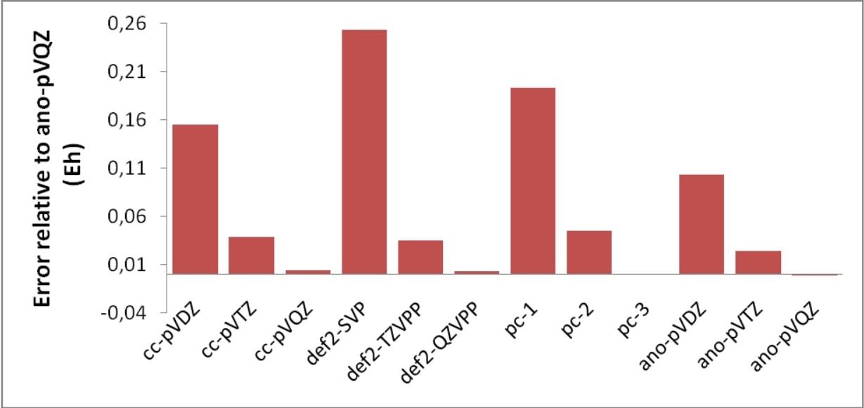
Fig. 3.7 Error in Eh for various basis sets for highly correlated calculations relative to the ano-pVQZ basis set.
Let us look at one more example in Table 3.39: the optimized structure of the N\(_2\) molecule as a function of basis set using the MP2 method (these calculations are a bit older from the time when the ano-pVnZ basis sets did not yet exist. Today, the ano-pVnZ would be preferred) .
The highest quality basis set here is QZVP and it also gives the lowest total energy. However, this basis set contains up to g-functions and is very expensive. Not using g-functions and a set of f-functions (as in TZVPP) has a noticeable effect on the outcome of the calculations and leads to an overestimation of the bond distance of 0.2 pm — a small change but for benchmark calculations of this kind still significant. The error made by the TZVP basis set that lacks the second set of d-functions on the bond distance, binding energy and ionization potential is surprisingly small even though the deletion of the second d-set “costs” more than 20 mEh in the total energy as compared to TZV(2d,2p), and even more compared to the larger TZVPP.
A significant error on the order of 1 – 2 pm in the calculated distances is produced by smaller DZP type basis sets, which underlines once more that such basis sets are really too small for correlated molecular calculations — the ANO-DZP basis sets are too strongly biased towards the atom, while the “usual” molecule targeted DZP basis sets like SVP have the d-set designed to cover polarization but not correlation (the correlating d-functions are steeper than the polarizing ones). The performance of the very economical SVP basis set should be considered as very good, and (a bit surprisingly) slightly better than cc-pVDZ despite that it gives a higher absolute energy.
Essentially the same picture is obtained by looking at the (uncorrected for ZPE) binding energy calculated at the MP2 level – the largest basis set, QZVP, gives the largest binding energy while the smaller basis sets underestimate it. The error of the DZP type basis sets is fairly large (\(\approx\) 2 eV) and therefore caution is advisable when using such bases.
Basis set |
R\(_{\mathbf{eq} }\) (pm) |
E(2N-N\(_{\mathbf{2} }\)) (eV) |
IP(N/N\(^{\mathbf{+} }\)) (eV) |
E(MP2) (Eh) |
|---|---|---|---|---|
SVP |
112.2 |
9.67 |
14.45 |
-109.1677 |
cc-pVDZ |
112.9 |
9.35 |
14.35 |
-109.2672 |
TZVP |
111.5 |
10.41 |
14.37 |
-109.3423 |
TZV(2d,2p) |
111.4 |
10.61 |
14.49 |
-109.3683 |
TZVPP |
111.1 |
10.94 |
14.56 |
-109.3973 |
QZVP |
110.9 |
11.52 |
14.60 |
-109.4389 |
3.10.6. The Coupled Cluster S-Diagnostic
There have been a number of diagnostic proposed for coupled cluster calculations that are designed to indicate “multi-reference” character. Unfortunately, the most widely used of them is the “T1-diagnostic”. We have argued for a long time, that the T1-diagnostic has nothing to do with multi-reference character. Rather, it measures the extent of orbital relaxation in the dynamic correlation field. While this is a measure of how good or bad the Hartree-Fock approximation works for the given system, it is expressis verbis NOT related to the multi-configuration character that the CC wavefunction may or may not want to emulate. For a discussion of what we consider as multi-reference versus single-reference character, please consult the paper by Izsak et al.
ORCA has an alternative coupled cluster diagnostic, known as the “S-diagnostic” that was introduced by Perdersen et al. This diagnostic does indeed measure multi-reference character. It is available for canonical RHF and UHF CCSD and is invoked by
%mdci DoSDiagnostic true
end
Relevant Papers:
Liakos, D. G.; Neese, F. Interplay of Correlation and Relativistic Effects in Correlated Calculations on Transition-Metal Complexes: The Cu₂O₂²⁺ Core Revisited. J. Chem. Theory Comput., 2011, 7, 1511–1523.
Izsák, Róbert; Ivanov, Aleksei V.; Blunt, Nick S.; Holzmann, Nicole; Neese, Frank. Measuring Electron Correlation: The Impact of Symmetry and Orbital Transformations. J. Chem. Theory Comput., 2023, 19 (10), 2703–2720. PMID: 37022051. DOI: 10.1021/acs.jctc.3c00122.
Faulstich, Fabian M.; Kristiansen, Håkon E.; Csirik, Mihaly A.; Kvaal, Simen; Pedersen, Thomas Bondo; Laestadius, Andre. S-Diagnostic─An a Posteriori Error Assessment for Single-Reference Coupled-Cluster Methods. The Journal of Physical Chemistry A, 2023, 127 (43), 9106–9120. PMID: 37874274. DOI: 10.1021/acs.jpca.3c01575.
3.10.8. Automatic extrapolation to the basis set limit
Note
This functionality is deprecated - it may still be usable but we will not actively maintain this part of code anymore. For basis set extrapolation please use the respective compound scripts.
As eluded to in the previous section, one of the biggest problems with correlation calculations is the slow convergence to the basis set limit. One possibility to overcome this problem is the use of explicitly correlated methods. The other possibility is to use basis set extrapolation techniques. Since this involves some fairly repetitive work, some procedures were hardwired into the ORCA program. So far, only energies are supported. For extrapolation, a systematic series of basis sets is required. This is, for example, provided by the cc-pV\(n\)Z, aug-cc-pV\(n\)Z or the corresponding ANO basis sets. Here \(n\) is the “cardinal number” that is 2 for the double-zeta basis sets, 3 for triple-zeta, etc.
The convergence of the HF energy to the basis set limit is assumed to be given by:
Here, \(E_{\mathrm{SCF} }^{(X) }\) is the SCF energy calculated with the basis set with cardinal number \(X\), \(E_{\mathrm{SCF} }^{(\infty) }\) is the basis set limit SCF energy and \(A\) and \(\alpha\) are constants. The approach taken in ORCA is to do a two-point extrapolation. This means that either \(A\) or \(\alpha\) have to be known. Here, we take \(A\) as to be determined and \(\alpha\) as a basis set specific constant.
The correlation energy is supposed to converge as:
The theoretical value for \(\beta\) is 3.0. However, it was found by Truhlar and confirmed by us, that for 2/3 extrapolations \(\beta = 2.4\) performs considerably better.
For a number of basis sets, we have determined the optimum values for \(\alpha\) and \(\beta\)[48]:
\(\alpha_{\mathbf{23} }\) |
\(\beta_{\mathbf{23} }\) |
\(\alpha_{\mathbf{34} }\) |
\(\beta_{\mathbf{34} }\) |
|
|---|---|---|---|---|
cc-pVnZ |
4.42 |
2.46 |
5.46 |
3.05 |
pc-n |
7.02 |
2.01 |
9.78 |
4.09 |
def2 |
10.39 |
2.40 |
7.88 |
2.97 |
ano-pVnZ |
5.41 |
2.43 |
4.48 |
2.97 |
saug-ano-pVnZ |
5.48 |
2.21 |
4.18 |
2.83 |
aug-ano-pVnZ |
5.12 |
2.41 |
Since the \(\beta\) values for 2/3 are close to 2.4, we always take this value. Likewise, all 3/4 and higher extrapolations are done with \(\beta=3\). However, the optimized values for \(\alpha\) are taken throughout.
Using the keyword ! Extrapolate(X/Y,basis), where X and Y are the
corresponding successive cardinal numbers and basis is the type of
basis set requested (= cc, aug-cc, cc-core, ano, saug-ano,
aug-ano, def2) ORCA will calculate the SCF and optionally the MP2 or
MDCI energies with two basis sets and separately extrapolate.
The keyword works also in the following way: ! Extrapolate(n,basis)
where n is the is the number of energies to be used. In this way the
program will start from a double-zeta basis and perform calculations
with n cardinal numbers and then extrapolate the different pairs of
basis sets. Thus for example the keyword ! Extrapolate(3,CC) will
perform calculations with cc-pVDZ, cc-pVTZ and cc-pVQZ basis sets and
then estimate the extrapolation results of both cc-pVDZ/cc-pVTZ and
cc-pVTZ/cc-pVQZ combinations.
Let us take the example of the H2O molecule at the B3LYP/TZVP optimized geometry. The reference values have been determined from a HF calculation with the decontracted aug-cc-pV6Z basis set and the correlation energy was obtained from the cc-pV5Z/cc-pV6Z extrapolation. This gives:
E(SCF,CBS)           = -76.066958 Eh
EC(CCSD(T),CBS)      =  -0.30866 Eh
Etot(CCSD(T),CBS)    = -76.37561 Eh
Now we can see what extrapolation can bring in:
!CCSD(T) Extrapolate(2/3) TightSCF Conv Bohrs
* int 0 1
O 0 0 0  0 0 0
H 1 0 0  1.81975 0 0
H 1 2 0  1.81975 105.237 0
*
NOTE:
The RI-JK and RIJCOSX approximations work well together with this option and RI-MP2 is also possible. Auxiliary basis sets are automatically chosen and can not be changed.
All other basis set choices, externally defined bases etc. will be ignored — the automatic procedure only works with the default basis sets!
The basis sets with the “core” postfix contain core correlation functions. By default it is assumed that this means that the core electrons are also to be correlated and the frozen core approximation is turned off. However, this can be overridden in the method block by choosing, e.g.
%method frozencore fc_electrons end!So far, the extrapolation is only implemented for single points and not for gradients. Hence, geometry optimizations cannot be done in this way.
The extrapolation method should only be used with very tight SCF convergence criteria. For open shell methods, additional caution is advised.
This gives:
Alpha(2/3)     :  4.420 (SCF Extrapolation)
Beta(2/3)      :  2.460 (correlation extrapolation)

SCF energy with basis cc-pVDZ:            -76.026430944
SCF energy with basis cc-pVTZ:            -76.056728252
Extrapolated CBS SCF energy (2/3) :       -76.066581429 (-0.009853177)

MDCI energy with basis cc-pVDZ:             -0.214591061
MDCI energy with basis cc-pVTZ:             -0.275383015
Extrapolated CBS correlation energy (2/3) : -0.310905962 (-0.035522947)

Estimated CBS total energy (2/3) :          -76.377487391
Thus, the error in the total energy is indeed strongly reduced. Let us look at the more rigorous 3/4 extrapolation:
Alpha(3/4)     :  5.460 (SCF Extrapolation)
Beta(3/4)      :  3.050 (correlation extrapolation)

SCF energy with basis cc-pVTZ:              -76.056728252
SCF energy with basis cc-pVQZ:              -76.064381269
Extrapolated CBS SCF energy (3/4) :         -76.066687152 (-0.002305884)

MDCI energy with basis cc-pVTZ:              -0.275383016
MDCI energy with basis cc-pVQZ:              -0.295324345
Extrapolated CBS correlation energy (3/4) :  -0.309520368 (-0.014196023)

Estimated CBS total energy (3/4) :           -76.376207520
In our experience, the ANO basis sets extrapolate similarly to the
cc-basis sets. Hence, repeating the entire calculation with
Extrapolate(3,ANO) gives:
Estimated CBS total energy (2/3) :           -76.377652792
Estimated CBS total energy (3/4) :           -76.376983433
Which is within 1 mEh of the estimated CCSD(T) basis set limit energy in the case of the 3/4 extrapolation and within 2 mEh for the 2/3 extrapolation.
For larger molecules, the bottleneck of the calculation will be the CCSD(T) calculation with the larger basis set. In order to avoid this expensive (or prohibitive) calculation, it is possible to estimate the CCSD(T) energy at the basis set limit as:
This assumes that the basis set dependence of MP2 and CCSD(T) is similar. One can then extrapolate as before. Alternatively, the standard way — as extensively exercised by Hobza and co-workers — is to simply use:
The appropriate keyword is:
! ExtrapolateEP2(2/3,ANO,MP2) TightSCF Conv Bohrs
* int 0 1
O 0 0 0  0 0 0
H 1 0 0  1.81975 0 0
H 1 2 0  1.81975 105.237 0
*
This creates the following output:
Alpha     :  5.410 (SCF Extrapolation)
Beta      :  2.430 (correlation extrapolation)

SCF energy with basis ano-pVDZ:              -76.059178452
SCF energy with basis ano-pVTZ:              -76.064774379
Extrapolated CBS SCF energy :                -76.065995735 (-0.001221356)

MP2 energy with basis ano-pVDZ:               -0.219202871
MP2 energy with basis ano-pVTZ:               -0.267058634
Extrapolated CBS correlation energy :         -0.295568604 (-0.028509970)

CCSD(T) correlation energy with basis ano-pVDZ: -0.229478341
CCSD(T) - MP2 energy with basis ano-pVDZ:       -0.010275470

Estimated CBS total energy :                   -76.371839809
The estimated correlation energy is not really bad — within 3 mEh from the basis set limit.
Using the ExtrapolateEP2(n/m,bas,[method, method-details]) keyword
one can use a generalization of the above method where instead of MP2
any available correlation method can be used as described in Ref.
[385]. method is optional and can be either MP2 or
DLPNO-CCSD(T), the latter being the default. In case the method is
DLPNO-CCSD(T) in the method-details option one can ask for LoosePNO,
NormalPNO or TightPNO.
Here M represents any correlation method one would like to use. For the previous water molecule the input of a calculation that uses DLPNO-CCSD(T) (which is the default now) instead of MP2 would look like:
! ExtrapolateEP2(2/3,cc,DLPNO-CCSD(T)) TightSCF Conv Bohrs
* int 0 1
O 0 0 0  0 0 0
H 1 0 0  1.81975 0 0
H 1 2 0  1.81975 105.237 0
*
and it would produce the following output:
Alpha     :  4.420 (SCF Extrapolation)
Beta      :  2.460 (correlation extrapolation)

SCF energy with basis cc-pVDZ:              -76.026430944
SCF energy with basis cc-pVTZ:              -76.056728252
Extrapolated CBS SCF energy :               -76.066581429 (-0.009853177)

MDCI energy with basis cc-pVDZ:              -0.214429497
MDCI energy with basis cc-pVTZ:              -0.275299699
Extrapolated CBS correlation energy :        -0.310868368 (-0.035568670)

CCSD(T) correlation energy with basis cc-pVDZ: -0.214548320
CCSD(T) - MDCI energy with basis cc-pVDZ:      -0.000118824

Estimated CBS total energy :                  -76.377568621
which is less than 2 mEh from the basis set limit. Finally it was shown [385] that instead of extrapolating the cheap method, M, using cardinal numbers \(X\) and \(X+1\) it is better to use cardinal numbers \(X+1\) and \(X+2\).
This can be done using the
ExtrapolateEP3(bas,[method,method-details]) keyword:
! ExtrapolateEP3(CC) TightSCF Conv Bohrs
and the corresponding output would be:
Alpha     :  5.460 (SCF Extrapolation)
Beta      :  3.050 (correlation extrapolation)

SCF energy with basis cc-pVDZ:               -76.026430944
SCF energy with basis cc-pVTZ:               -76.056728252
SCF energy with basis cc-pVQZ:               -76.064381269
Extrapolated CBS SCF energy :                -76.066687152 (-0.002305884)

MDCI energy with basis cc-pVDZ:               -0.214429497
MDCI energy with basis cc-pVTZ:               -0.275299699
MDCI energy with basis cc-pVQZ:               -0.295229871
Extrapolated CBS correlation energy :         -0.309417951 (-0.014188080)

CCSD(T) correlation energy with basis cc-pVDZ: -0.214548319
CCSD(T) - MDCI energy with basis cc-pVDZ:      -0.000118822

Estimated CBS total energy :                  -76.376223926
For the ExtrapolateEP2, and ExtrapolateEP3 keywords the default cheap method is the DLPNO-CCSD(T) with the NormalPNO thresholds. There also available options with MP2, and DLPNO-CCSD(T) with LoosePNO and TightPNO settings.
3.10.9. Cluster in molecules (CIM)
Cluster in molecules (CIM) approach is a linear scaling local correlation method developed by Li and the coworkers in 2002.[386] It was further improved by Li, Piecuch, Kállay and other groups recently.[387, 388, 389, 390, 391] The CIM is inspired by the early local correlation method developed by Förner and coworkers.[392] The total correlation energy of a closed-shell molecule can be considered as a summation of correlation energies of each occupied LMOs.
For each occupied LMO, it only correlates with its nearby occupied LMOs and virtual MOs. To reproduce the correlation energy of each occupied LMO, only a subset of occupied and virtual LMOs are needed in the correlation calculation. Instead of doing the correlation calculation of the whole molecule, the correlation energies of all LMOs can be obtained within various subsystems.
The CIM approach implemented in ORCA is following an algorithm proposed by Guo and coworkers with a few improvements.[390, 391]
To avoid the real space cutoff, the differential overlap integral (DOI) is used instead of distance threshold. There is only one parameter ‘CIMTHRESH’ in CIM approach, controlling the construction of CIM subsystems. If the DOI between LMO i and LMO j is larger than CIMTHRESH, LMO j will be included into the MO domain of i. By including all nearby LMO of i, one can construct a subsystem for MO i. The default value of CIMTHRESH is 0.001. If accurate results are needed, a tighter CIMTHRESH must be used.
Since ORCA 4.1, the neglected correlations between LMO i and LMOs outside the MO domain of i are considered as well. These weak correlations are approximately evaluated by dipole moment integrals. With this correction, the CIM results of 3 dimensional proteins are significantly improved. About 99.8% of the correlation energies are recovered.
The CIM can invoke different single reference correlation methods for
the subsystem calculations. In ORCA the CIM-RI-MP2, CIM-CCSD(T),
CIM-DLPNO-MP2 and CIM-DLPNO-CCSD(T) methods are available. The CIM-RI-MP2 and
CIM-DLPNO-CCSD(T) have been proved to be very efficient and accurate
methods to compute correlation energies of very big molecules,
containing a few thousand atoms.[391]
The usage of CIM in ORCA is simple. For CIM-RI-MP2,
#
# CIM-RI-MP2 calculation
#
! RI-MP2 cc-pVDZ cc-pVDZ/C CIM
%CIM
  CIMTHRESH 0.0005  # Default value is 0.001
end

* xyzfile 0 1 CIM.xyz
For CIM-DLPNO-CCSD(T),
#
# CIM-DLPNO-CCSD calculation
#
! DLPNO-CCSD(T) cc-pVDZ  cc-pVDZ/C CIM
* xyzfile 0 1 CIM.xyz
The parallel efficiency of CIM has been significantly improved.[391] Except for a few domain construction sub-steps, the CIM algorithm can achieve very high parallel efficiency. Since ORCA 4.1, the parallel version does not support Windows platform anymore due to the parallelization strategy. The generalization of CIM from closed-shell to open-shell (multi-reference) will also be implemented in the near future.
3.10.10. Local correlation (DLPNO)
ORCA features the extremely powerful “domain-based local pair natural orbital” approximation (DLPNO),[393] which is an extension of the “local pair natural orbital” ansatz (LPNO).[379, 380, 381, 394] These methods are designed to provide results as close as possible to the canonical coupled-cluster results while gaining orders of magnitude of efficiency through a series of well-controlled approximations. In fact, typically about 99.8% to 99.9% of the canonical correlation energy is recovered in such calculations. Even higher accuracy is achievable but will ultimately come at much higher computational cost. The default cut-offs are set such that the vast majority of chemically meaningful energy differences are reproduced to better than 1 kcal/mol relative to the canonical results with the same basis set.
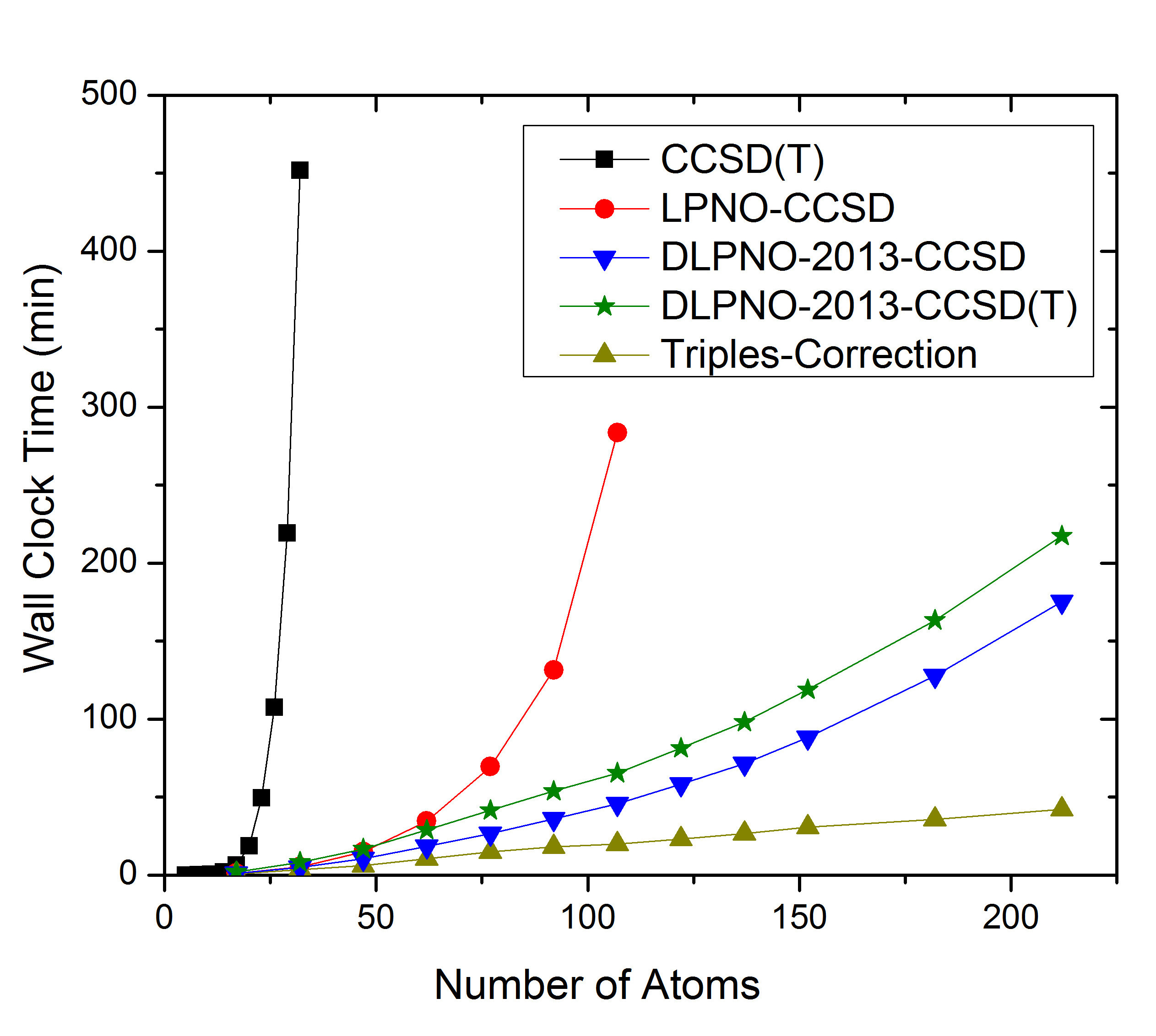
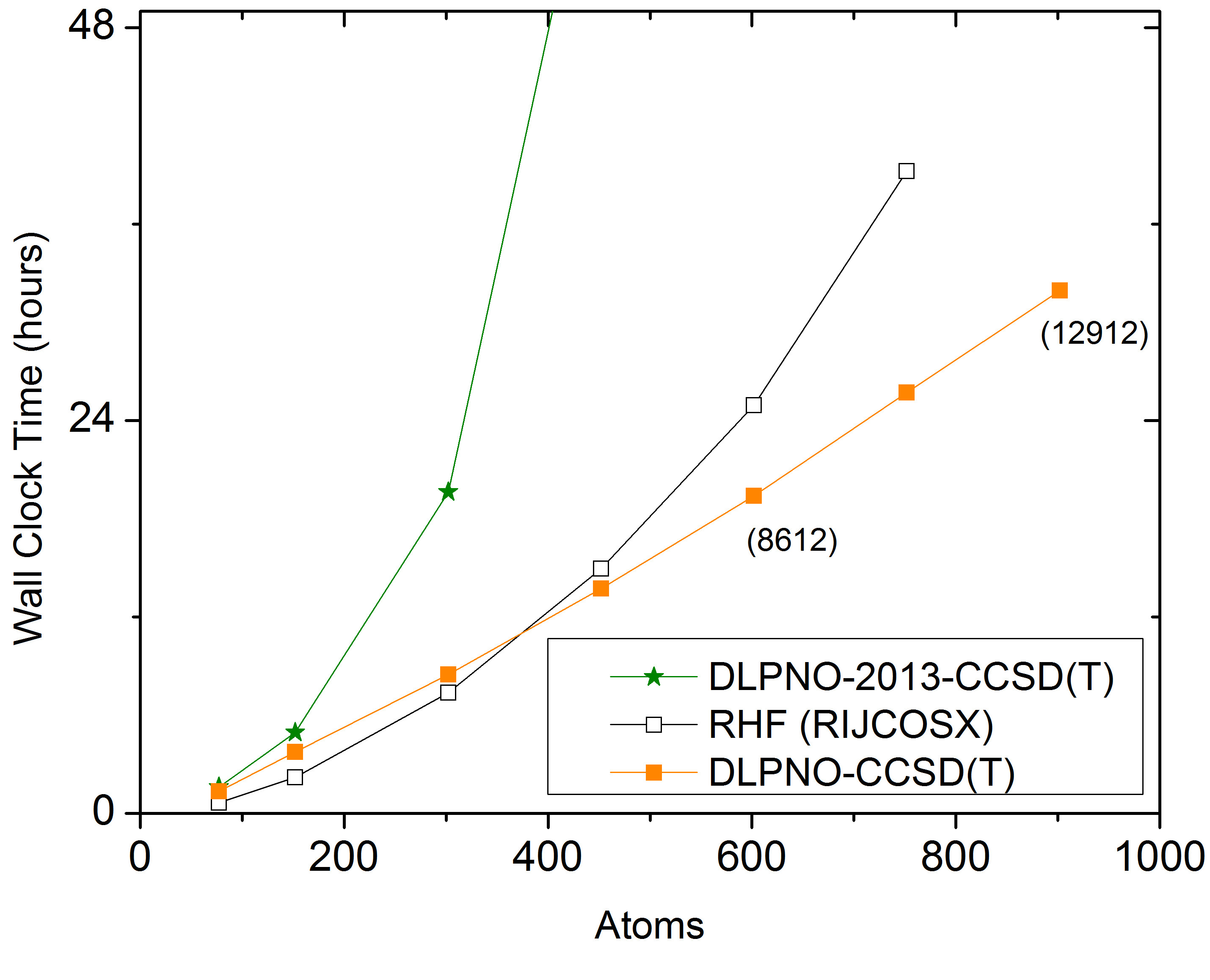
With ORCA 6.0, the LPNO variants are no longer supported, as they involve some higher order scaling steps (up to \(N^5\)) while DLPNO is linear scaling and of similar accuracy. The comparison between LPNO-CCSD and DLPNO-CCSD is shown in Fig. 3.8. It is obvious that DLPNO-CCSD is (almost) never slower than LPNO-CCSD. However, its true advantages do become most apparent for molecules with more than approximately 60 atoms. The triples correction, that was added with our second paper from 2013, shows a perfect linear scaling, as is shown in part (a) of Fig. 3.8. For large systems it adds about 10%–20% to the DLPNO-CCSD computation time, hence its addition is possible for all systems for which the latter can still be obtained. Since 2016, the entire DLPNO-CCSD(T) algorithm is linear scaling. The improvements of the linear-scaling algorithm, compared to DLPNO2013-CCSD(T), start to become significant at system sizes of about 300 atoms, as becomes evident in part (b) of Fig. 3.8.
 (a) DLPNO2013 Scaling
 (b) DLPNO Scaling
Fig. 3.8 a) Scaling behavior of the canonical CCSD, LPNO-CCSD and DLPNO2013-CCSD(T) methods. It is obvious that only DLPNO2013-CCSD and DLPNO2013-CCSD(T) can be applied to large molecules. The advantages of DLPNO2013-CCSD over LPNO-CCSD do not show before the system has reached a size of about 60 atoms. b) Scaling behavior of DLPNO2013-CCSD(T), DLPNO-CCSD(T) and RHF using RIJCOSX. It is obvious that only DLPNO-CCSD(T) can be applied to truly large molecules, is faster than the DLPNO2013 version, and even has a crossover with RHF at about 400 atoms.
Using the DLPNO-CCSD(T) approach it was possible for the first time (in 2013) to perform a CCSD(T) level calculation on an entire protein (Crambin with more than 650 atoms, Fig. 3.9). While the calculation using a double-zeta basis took about 4 weeks on one CPU with DLPNO2013-CCSD(T), it takes only about 4 days to complete with DLPNO-CCSD(T). With DLPNO-CCSD(T) even the triple-zeta basis calculation can be completed within reasonable time, taking 2 weeks on 4 CPUs.
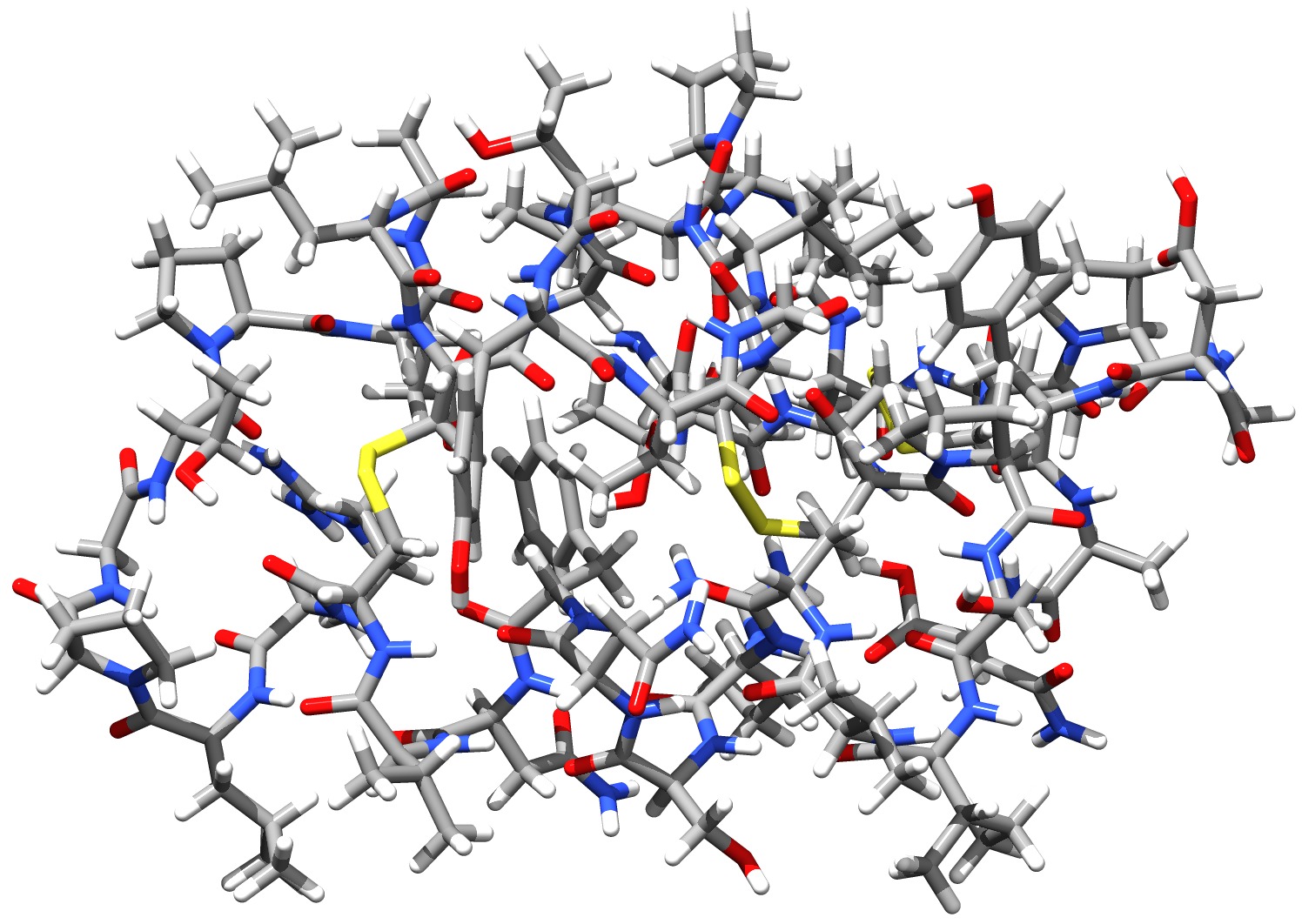
Fig. 3.9 Structure of the Crambin protein - the first protein to be treated with a CCSD(T) level ab initio method
It is important to understand that the LPNO and DLPNO implementations are intimately tied to the RI approximation. Hence, in these calculations one must specify a fitting basis set. The same rules as for RI-MP2 apply: the auxiliary basis sets optimized for MP2 are just fine for PNO calculations. You can specify several aux bases for the same job and the program will sort it out correctly.
The theory of the LPNO and DLPNO methods has been thoroughly described in the literature in a number of original research papers:
F. Neese, A. Hansen, D. G. Liakos: Efficient and accurate local approximations to the coupled-cluster singles and doubles method using a truncated pair natural orbital basis.[379]
F. Neese, A. Hansen, F. Wennmohs, S. Grimme: Accurate Theoretical Chemistry with Coupled Electron Pair Models.[381]
F. Neese, F. Wennmohs, A. Hansen: Efficient and accurate local approximations to coupled electron pair approaches. An attempt to revive the pair-natural orbital method.[394]
D. G. Liakos, A. Hansen, F. Neese: Weak molecular interactions studied with parallel implementations of the local pair natural orbital coupled pair and coupled-cluster methods.[395]
A. Hansen, D. G. Liakos, F. Neese: Efficient and accurate local single reference correlation methods for high-spin open-shell molecules using pair natural orbitals.[380]
C. Riplinger, F. Neese: An efficient and near linear scaling pair natural orbital based local coupled-cluster method.[393]
C. Riplinger, B. Sandhoefer, A. Hansen, F. Neese: Natural triple excitations in local coupled-cluster calculations with pair natural orbitals.[396]
C. Riplinger, P. Pinski, U. Becker, E. F. Valeev, F. Neese: Sparse maps - A systematic infrastructure for reduced-scaling electronic structure methods. II. Linear scaling domain based pair natural orbital coupled cluster theory.[397]
D. Datta, S. Kossmann, F. Neese: Analytic energy derivatives for the calculation of the first-order molecular properties using the domain-based local pair-natural orbital coupled-cluster theory[398]
M. Saitow, U. Becker, C. Riplinger, E. F. Valeev, F. Neese: A new linear scaling, efficient and accurate, open-shell domain based pair natural orbital coupled cluster singles and doubles theory.[399]
Y. Guo, C. Riplinger, U. Becker, D.G. Liakos, Y. Minenkov, L. Cavallo, and F. Neese: An improved linear scaling perturbative triples correction for the domain based local pair-natural orbital based singles and doubles coupled cluster method (DLPNO-CCSD(T)).[400]
Hence, it is sufficient to only point to a few significant design principles and features of these methods:
The correlation energy of any molecule can be written as a sum over the correlation energies of pairs of electrons, labelled by the internal indices (\(ij\)) of pairs of orbitals that are occupied in the reference determinant. If the orbitals (\(i\)) and (\(j\)) are localized, the pair correlation energy \(\epsilon_{ij}\) falls off very quickly with distance, quite typically by about an order of magnitude per chemical bond that is separating orbitals (\(i\)) and (\(j\)). Hence, by using a suitable cut-off for a reasonable pair correlation energy estimate many electron pairs can be removed from the high-level treatment and only a linear scaling number of electron pairs will make a significant contribution to the correlation energy.
The natural estimate for the pair correlation energy comes from second order many body perturbation theory (MP2). However, canonical MP2 is scaling with the fifth power of the molecular size and hence, is not really attractive from a theoretical nor computational point of view. Owing to the small pre-factor RI-MP2 goes a long way to provide reasonably cheap estimates for pair correlation energies. However, if one uses localized internal orbitals, then the MP2 energy expression must be cast in form of linear equations. On the other hand, if one uses canonical virtual orbitals together with localized internal orbitals and neglects the coupling terms coming from purely internal Fock matrix elements F(\(i\),\(k\)) and F(\(k\),\(j\)) then one ends up with a fair approximation that is termed “semi-canonical MP2” in ORCA. It serves as a guess in the older LPNO method. For DLPNO this method is also not attractive.
In DLPNO, the guess is more sophisticated. Here the virtual space is spanned by projected atomic orbitals (PAOs) that are assigned to domains of atoms that are associated with each local internal orbital (\(i\)) and with the union of two such domains (\(i\)) and (\(j\)) for the electron pair (\(ij\)). If one applies the semi-local approximation, one obtains an excellent approximation to the semi-canonical MP2 energy. This is called the “semi-local” approximation and it scales linearly with respect to computational effort. If one iterates these equations to self-consistency to eliminate the coupling terms F(\(i\),\(k\)) and F(\(k\),\(j\)) then one obtains the full local MP2 method (LMP2 or L-MP2). By making the domains large enough the results approach the canonical MP2 energy to arbitrary accuracy while still being linear scaling with respect to computational resources. This method is the default for the DLPNO method.
Basically, the high-spin open-shell version of the DLPNO uses the same strategy as the closed-shell variant to efficiently generate the open-shell PNOs in a consistent manner to the closed-shell formalism. Through the development of the UHF-LPNO-CCSD method, we have realized that use of the unrestricted MP2 (UMP2) approach to define the open-shell PNOs introduces a few complexities; (1) the PNOs for \(\beta\) spin orbitals cannot be defined for \(\alpha\)-\(\alpha\) electron pairs and vice versa, (2) the diagonal PNOs for singly occupied orbitals cannot be properly defined, and (3) the PNO space does not become identical to that in the closed-shell LPNO framework in the closed-shell limit. However, to program all the unrestricted CCSD terms in the LPNO basis, those PNOs are certainly necessary. Therefore, in the UHF-LPNO-CCSD implementation, several terms, which, in many cases, give rather minor contributions in the correlation energy are omitted. Due to these facts, the UHF-LPNO-CCSD does not give identical results to that of RHF-LPNO-CCSD in the closed-shell limit. In addition, screening of the weak pairs on the basis of the semi-canonical UMP2 pair-energy results in somewhat unbalanced treatment of the closed- and open-shell states in some cases, leading to rather larger errors in the reaction energies. To overcome those issues, in the high-spin open-shell DLPNO-CCSD method, the PNOs are generated in the framework of semi-canonical NEVPT2 which smoothly converges to the RHF-MP2 counterpart in the closed-shell limit. The open-shell DLPNO-CCSD, which is made available from ORCA 4.0, includes a full set of the open-shell CCSD equations and is designed as a natural extension to the RHF-DLPNO-CCSD.
Screening of the electron pairs according to a truncation parameter (in ORCA it is called \(T_\mathrm{CutPairs}\)) is not sufficient to obtain a highly performing local electronic structure method. The original work of Pulay suggested to limit excitations out of the internal orbitals (\(i\)) and (\(j\)) to the domain associated with the pair (\(ij\)). While this works well and has been implemented to perfection by Werner, Schütz and co-workers over the years,[401, 402, 403, 404] the pre-factor of such calculations is high, since the domains have to be chosen large in order to recover 99.9% or more of the canonical correlation energy.
The ORCA developers have therefore turned to an approach that has been used with a high degree of success in the early 1970s by Meyer, Kutzelnigg, Staemmler and their co-workers, namely the method of “pair natural orbitals” (PNOs).[405, 406, 407, 408]
As shown by Loewdin in his seminal paper from 1955, natural orbitals (the eigenfunctions of the one-particle density matrix) provide the fastest possible convergence of the correlated wavefunction with respect to the number of one-particle functions included in the virtual space. It has been amply established that approximate natural orbitals are almost as succesful as the true natural orbitals (which would require the knowledge of the exact wavefunction) in this respect. While the success of approximate correlation treatments of many particle systems that use approximate natural orbitals of the whole systems are somewhat limited, this is not the case for pair natural orbitals. The latter have first been suggested as a basis for correlation calculations by England and co-workers and, at the time, were given the name “pseudonatural orbitals”, a term that was used by Meyer throughout his pioneering work.The PNOs are approximate natural orbitals of a given electron pair. In order to generate them one requires a one particle pair density matrix \(D_{ij}\) the eigenfunctions of which are the PNOs themselves while the corresponding eigenvalues are the PNO occupation numbers. While there are many creative possibilities that can lead to slightly different PNO sets, a quite useful and natural approximation is to generate such a density from the MP2 amplitudes as an expectation value (the “unrelaxed” MP2 density. One then uses a second threshold (in ORCA\(T_\mathrm{CutPNO}\)) that controls the PNOs to be included in the calculation. PNOs with an occupation number \(< T_\mathrm{CutPNO}\) are neglected.
PNOs of a given electron pair form an orthonormal set. However, PNOs belonging to different electron pairs are not orthonormal and hence they overlap. This non-orthogonality leads to surprisingly few complications because the PNOs stay orthogonal to all occupied orbitals. In practice, the equations for PNO-based correlation calculations are hardly more complex than the canonical equations.
The nice feature of these pair densities is that they become small when the pair interaction becomes small. Hence weak pairs are correlated by very few PNOs. Therefore, the PNO expansion of the wavefunction is extremely compact and there only is a linear scaling number of significant excitation amplitudes that need to be considered.
A great feature of the PNOs is that they are “self-adapting” to the correlation situation that they are supposed to describe. Hence, they are as delocalized as required by the physics and there is no ad-hoc assumption about their location in space. However, it is clear that the PNOs are located in the same region of space as the internal orbitals that they correlate because otherwise they would not contribute to the correlation energy.
In the iterative local MP2, a set of PNOs is calculated for the MP2 calculation from the semicanonical amplitudes first using the cutoff
TCutPNO\(\times\)LMP2ScaleTCutPNO. The size of the resulting PNO space should be comparable with DLPNO-MP2. After the iterations have converged, a (smaller) set of PNOs for the CCSD double excitation amplitudes is generated from the iterated local MP2 amplitudes in the (larger) PNO basis. The PNOs for the single excitation amplitudes are always calculated using the semicanonical MP2 amplitudes, as they require a much more conservative PNO truncation threshold.Capitalizing on this feature one can define generous domains and expand the PNOs in terms of the PAOs and auxiliary fit functions (for the RI approximations) that are contained in these domains. In ORCA this is controlled by the third significant truncation parameter \(T_\mathrm{CutMKN}\). This is the basis of the DLPNO method. In the older LPNO method, the PNOs are expanded in terms of the canonical virtual orbitals and \(T_\mathrm{CutMKN}\) is only used for a local fit to the PNOs. In the linear-scaling DLPNO implementation the domains expanding the PNOs in terms of the PAOs are controlled via \(T_\mathrm{CutDO}\).
PNO expansions have the amazing advantage that the PNOs converge to a well-defined set as the basis set is approaching completeness. Hence, the increase in the number of PNOs per electron pair is very small upon enlargement of the orbital basis. In other words, correlation calculations with large basis sets are not that much more expensive than correlation calculations with small basis sets. Thus, the advantage of PNO over canonical calculations increases with the size of the basis set. This is a great feature as large and flexible basis sets are a requirement for meaningful correlation calculations.
In summary, DLPNO and LPNO calculations are controlled by only three cut-off parameters with well-defined meanings: a) \(T_\mathrm{CutPairs}\), the cut-off for the electron pairs to be included in the coupled-pair or coupled-cluster iterations, b) \(T_\mathrm{CutPNO}\) which controls how many PNOs are retained for a given electron pair and c) \(T_\mathrm{CutMKN}\) that controls how large the domains are that the PNOs expand over. For the linear-scaling DLPNO calculations the domain sizes are controlled via \(T_\mathrm{CutDO}\).
It is clear that owing to the truncations a certain amount of error is introduced in the results. However, having the LMP2 results available, one can compensate for the errors coming from \(T_\mathrm{CutPairs}\) and \(T_\mathrm{CutPNO}\). This is done in ORCA and the correction is added to the final correlation energy, thus bringing it very close (to mEh accuracy or better) to the canonical result. \(T_\mathrm{CutMKN}\) is best dealt with by making it conservative (at 1e\(-\)3 to 1e\(-\)4 the domains are about 20–30 atoms large, which is sufficient for an accurate treatment).
Note that the LPNO and DLPNO methods do not introduce any real space cut-offs. We refrain from doing so and insist in our method development by making all truncations based on wavefunction or energy parameters. We feel that this is the most unbiased approach and it involves no element of “chemical intuition” or “prejudice”.
In the DLPNO method a highly efficient screening mechanism is operative. In this method one first obtains a (quadratically scaling) multipole estimate for the pair correlation energy that is extremely fast to compute (a few seconds, even for entire proteins). Only if this estimate is large enough, a given electron pair is even considered for a LMP2 treatment. Quite typically pairs with energy contributions of 1e\(-\)6 Eh and smaller are very well described by the dipole-dipole estimate. Specifically, we drop pairs with estimated energies \(< 0.01 \times T_\mathrm{CutPairs}\) and add their multipole energy sum to the final correlation energy. These corrections tend to be extremely small, even for large molecules and are insignificant for the energy. However, importantly, the multipole estimate ensures linear scaling in the MP2 treatment. The pairs that then do not survive the pair-prescreening are called “weak pairs” in the ORCA or DLPNO sense. They still play a role in the calculation of the triple excitation correction.
The calculation of triple excitation contributions is more involved and one does not have a perturbative estimate available since the (T) contribution is perturbative itself. While the (T) contribution is much smaller than the CCSD correlation energy, the errors introduced by the various local and PNO approximations can be significant. We found that one has to include triples with at least one pair being a “weak” LMP2 pair (with its LMP2 amplitudes) in order to arrive at sufficiently accurate results.
3.10.10.1. Basic Usage
The use of the DLPNO methods is simple and requires little special attention from the user:
# Local Pair Natural Orbital Test
! cc-pVTZ cc-pVTZ/C DLPNO-CCSD TightSCF
%maxcore 2000

# these are the default values - they need not to be touched!
%mdci  TCutPNO   3.33e-7   # cutoff for PNO occupation numbers. This
                           # is the main truncation parameter
       TCutPairs 1e-4  # cut-off for estimated pair correlation energies.
                       # This exploits the locality in the internal space
       TCutMKN   1e-3  # this is a technical parameter here that controls
                       # the domain size for the local fit to the PNOs.
		       # It is conservative.
       end

* xyz 0 1
... (coordinates)
*
The LPNO methods used to run in strict analogy to their canonical variants. In fact, one should not view the LPNO methods as new model chemistry - they are designed to reproduce the canonical results, including BSSE. This is different from the domain based local correlation methods that do constitute a new model chemistry with properties that are different from the original methods.
In some situations, it may be appropriate to adapt the accuracy of the calculation. Sensible defaults have been determined from extensive benchmark calculations and are accessible via LoosePNO, NormalPNO and TightPNO keywords in the simple input line.[409]
These keywords represent the recommended way to control the accuracy of DLPNO calculations as follows. Manual changing of thresholds beyond these specifying these keywords is usually discouraged.
# Tight settings for increased accuracy, e.g. when investigating
# weak interactions or conformational equilibria
! cc-pVTZ cc-pVTZ/C DLPNO-CCSD(T) TightPNO TightSCF

# OR: Default settings (no need to give NormalPNO explicitly)
# Useful for general thermochemistry
! cc-pVTZ cc-pVTZ/C DLPNO-CCSD(T) NormalPNO TightSCF

# OR: Loose settings for rapid estimates
! cc-pVTZ cc-pVTZ/C DLPNO-CCSD(T) LoosePNO TightSCF

%maxcore 2000

* xyz 0 1
... (coordinates)
*
Since ORCA 4.0, the linear-scaling DLPNO implementation described in reference [397] is the default DLPNO algorithm. However, for comparison, the first DLPNO implementation from references [393] and [396] can still be called by using the DLPNO2013 prefix instead of the DLPNO- prefix.
# DLPNO-CCSD(T) calculation using the 2013 implementation
! cc-pVTZ cc-pVTZ/C DLPNO2013-CCSD(T)

# DLPNO-CCSD(T) calculation using the linear-scaling implementation
! cc-pVTZ cc-pVTZ/C DLPNO-CCSD(T)

* xyz 0 1
... (coordinates)
*
Until ORCA 4.0, the “semi-canonical” approximation is used in the perturbative triples correction for DLPNO-CCSD. It was found that the “semi-canonical” approximation is a very good approximation for most systems. However, the “semi-canonical” approximation can introduce large errors in rare cases (particularly when the HOMO-LUMO gap is small), whereas the DLPNO-CCSD is still very accurate. To improve the accuracy of perturbative triples correction, since 4.1, an improved perturbative triples correction for DLPNO-CCSD is available, DLPNO-CCSD(T1)[400]. In DLPNO-CCSD(T1), the triples amplitudes are computed iteratively, which can reproduce more accurately the canonical (T) energies.
It is necessary to clarify the nomenclature used in ORCA input files. The keyword to invoke “semi-canonical” perturbative triples correction approximation is DLPNO-CCSD(T). While, the keyword of improved iterative approximation is DLPNO-CCSD(T1). However, in our recent paper[400], the “semi-canonical” perturbative triples correction approximation is named DLPNO-CCSD(T0), whereas the improved iterative one is called DLPNO-CCSD(T). Thus, the names used in our paper are different from those in ORCA input files. An example input file to perform improved iterative perturbative triples correction for DLPNO-CCSD is given below,
# DLPNO-CCSD(T1) calculation using the iterative triples correction
! cc-pVTZ cc-pVTZ/C DLPNO-CCSD(T1)

%mdci
      TNOSCALES  10.0 #TNO truncation scale for strong triples,
                      # TNOSCALES*TCutTNO. Default setting is 10.0
      TNOSCALEW 100.0 #TNO truncation scale for weak triples,
                      # TNOSCALEW*TCutTNO Default setting is 100.0
      TriTolE    1e-4 #(T) energy convergence tolerance
                      # Default setting is 1e-4
%end
* xyz 0 1
... (coordinates)
*
Since ORCA 4.2, the improved iterative perturbative triples correction for open-shell DLPNO-CCSD is available as well. The keyword of open-shell DLPNO-CCSD(T) is the same as that of the closed-shell case.
Since ORCA 4.0, the high-spin open-shell version of the DLPNO-CISD/QCISD/CCSD implementations have been made available on top of the same machinery as the 2016 version of the RHF-DLPNO-CCSD code. The present UHF-DLPNO-CCSD is designed to be an heir to the UHF-LPNO-CCSD and serves as a natural extension to the RHF-DLPNO-CCSD. A striking difference between UHF-LPNO and newly developed UHF-DLPNO methods is that the UHF-DLPNO approach gives identical results to that of the RHF variant when applied to closed-shell species while UHF-LPNO does not. Usage of this program is quite straightforward and shown below:
# (1) In case of ROHF reference
! ROHF DLPNO-CCSD def2-TZVPP def2-TZVPP/C TightSCF TightPNO

# (2) In case of UHF reference, the QROs are constructed first and used for
#     the open-shell DLPNO-CCSD computations
! UHF DLPNO-CCSD def2-TZVPP def2-TZVPP/C TightSCF TightPNO

# (3) In case that UKS is specified, the QROs are constructed first and used as
#     "unconverged" UHF orbitals for the open-shell DLPNO-CCSD computations.
#     This approach is useful when the converged UHF wavefunction is qualitatively
#     wrong but the UKS wavefunction is not
! UKS CAM-B3LYP DLPNO-CCSD def2-TZVPP def2-TZVPP/C TightSCF TightPNO
Note
DLPNO-CISD/QCISD/CCSD methods are dedicated to closed-shell and high-spin open-shell species, but not spin-polarized systems (e.g. open shell singlets or antiferromagnetically coupled transition metal clusters). Performing DLPNO-CISD/QCISD/CCSD calculations upon open shell singlet UHF/UKS wavefunctions will give results resembling the corresponding closed shell singlet calculations, because the DLPNO calculations will be done on the closed-shell determinant composed of the QRO orbitals. Similarly, calculations of spin-polarized systems other than open shell singlets may give qualitatively wrong results. Here, the UHF-LPNO-CCSD method or the DLPNO-NEVPT2 are better alternatives.
The same set of truncation parameters as closed-shell DLPNO-CCSD is used also in case of open-shell DLPNO. The open-shell DLPNO-CCSD produces more than 99.9 \(\%\) of the canonical CCSD correlation energy as in case of the closed-shell variant. The computational timings of the UHF-DLPNO-CCSD and RIJCOSX-UHF for linear alkane chains in triplet state are shown in Fig. 3.10.

Fig. 3.10 Computational times of RIJCOSX-UHF and UHF-DLPNO-CCSD for the linear alkane chains (\(C_{n}H_{\text{2n + 2}}\)) in triplet state with def2-TZVPP basis and default frozen core settings. 4 CPU cores and 128 GB of memory were used on a single cluster node.
Although those systems are somewhat idealized for the DLPNO method to best perform, it is clear that the preceding RIJCOSX-UHF is the rate-determining step in the total computational time for large examples. In the open-shell DLPNO implementations, SOMOs are included not only in the occupied space but also in the PNO space in the preceding integral transformation step. This means the presence of more SOMOs may lead to more demanding PNO integral transformation and DLPNO-CCSD iterations. The illustrative examples include active site model of the [NiFe] Hydrogenase in triplet state and the oxygen evolving complex (OEC) in the high-spin state, which are shown in Figures 7 and 8, respectively. With def2-TZVPP basis set and NormalPNO settings, a single point calculation on [NiFe] Hydrogenase (Fig. 3.11) took approximately 45 hours on a single cluster node by using 4 CPU cores of Xeon E5-2670. A single point calculation on the OEC compound (Fig. 3.12) with the same computational settings finished in 44 hours even though the number of AOs in this system is even fewer than the Hydrogenase: the Hydrogenase active site model and OEC involve 4007 and 2606 AO basis functions, respectively. Special care should be taken if the system possesses more than ten SOMOs, since inclusion of more SOMOs may drastically increase the prefactor of the calculations. In addition, if the SOMOs are distributed over the entire molecular skeleton, each pair domain may not be truncated at all; in this case speedup attributed to the domain truncation will not be achieved at all.

Fig. 3.11 Ni-Fe active center in the [NiFe] Hydrogenase in its second-coordination sphere. The whole model system is composed of 180 atoms.

Fig. 3.12 A model compound for the OEC in the S\({}_2\) state of photosystem II which is composed of 238 atoms. In its high-spin state, the OEC possesses 13 SOMOs in total.
Calculation of the orbital-unrelaxed density has been implemented for closed-shell DLPNO-CCSD. This permits analytical computation of first-order properties, such as multipole moments or electric field gradients. In order to reproduce conventional unrelaxed CCSD properties to a high degree of accuracy, tighter thresholds may be needed than given by the default settings. Reading of the reference[398] is recommended. Calculation of the unrelaxed density is requested as usual:
%MDCI Density Unrelaxed End
There are a few things to be noticed about (D)LPNO methods:
The DLPNO and LPNO methods obligatorily make use of the RI approximation. Hence, a correlation fit set must be provided.
The DLPNO-CCSD(T) method is applicable to closed-shell or high-spin open-shell species. When performing DLPNO calculations on open-shell species, it is always better to have UCO option: If preceding SCF converges to broken-symmetry solutions, it is not guaranteed that the DLPNO-CCSD gives physically meaningful results.
The open-shell version of the DLPNO approach uses a different strategy to the LPNO variant to define the open-shell PNOs. This ensures that, unlike the open-shell LPNO, the PNO space converges to the closed-shell counterpart in the closed-shell limit. Therefore, in the closed-shell limit, the open-shell DLPNO gives identical correlation energy to the RHF variant up to at least the third decimal place. The perturbative triples correction referred to as, (T), is also available for the open-shell species.
When performing a calculation on the open-shell species with either of canonical/DLPNO methods on top of the Slater determinant constructed from the QROs, special attention should be paid on the orbitals energies of those QROs. In some cases, the orbitals energy of the highest SOMO appear to be higher than that of the lowest VMO. Similarly to this, the orbital energy of the highest DOMO may appear to higher than that of the lowest SOMOs. In such cases, the CEPA/QCISD/CCSD iteration may show difficulty in convergence. In the worst case, it just diverges. Most likely, in such cases, one has to suspect the charge and multiplicity might be wrong. If they are correct, you may need much prettier starting orbitals and a bit of good luck! Apart from a careful choice of starting orbitals (in particular, DFT orbitals can be used in place of the default HF orbitals if the latter have qualitative deficiencies, including but not limited to severe spin contamination), changing the maximum DIIS expansion space size (
MaxDIIS) and the level shift (LShift) in the%mdciblock may alleviate the convergence problems to some extent.DLPNO-CCSD(T)-F12 and DLPNO-CCSD(T1)-F12 (iterative triples) are available for both closed- and open-shell cases. These methods employ a perturbative F12 correction on top of the DLPNO-CCSD(T) correlation energy calculation. The F12 part of the code uses the RI approximation in the same spirit as the canonical RI-F12 methods (refer to section Explicitly Correlated Methods: F12-MP2 and F12-CCSD(T)). Hence, they should be compared with methods using the RI approximation for both CC and F12 parts. The F12 correction takes only a fraction (usually 10-30%) of the total time (excluding SCF) required to calculate the DLPNO-CCSD(T)-F12 correlation energy. Thus, the F12 correction scales the same (linear or near-linear) as the parent DLPNO method. Furthermore, no new truncation parameters are introduced for the F12 procedure, preserving the black-box nature of the DLPNO method. The F12D approximation is highly recommended as it is computationally cheaper than the F12 approach which involves a double RI summation. Keywords: DLPNO-CCSD(T)-F12D, DLPNO-CCSD(T)-F12, DLPNO-CCSD(T1)-F12D, DLPNO-CCSD(T1)-F12, DLPNO-CCSD-F12D, DLPNO-CCSD-F12.
There are three thresholds that can be user controlled that can all be adjusted in the %mdci block: (a) \(T_\text{CutPNO}\hspace{-0.25mm}\) controls the number of PNOs per electron pair. This is the most critical parameter and has a default value of \(3.33\times 10^{-7}\). (b) \(T_\text{CutPairs}\hspace{-0.25mm}\) controls a perturbative selection of significant pairs and has a default value of \(10^{-4}\). (c) \(T_\text{CutMKN}\hspace{-0.25mm}\) is a technical parameter and controls the size of the fit set for each electron pair. It has a default value of \(10^{-3}\). All of these default values are conservative. Hence, no adjustment of these parameters is necessary. All DLPNO-CCSD truncations are bound to these three truncation parameters and should almost not be touched (Hence they are also not documented :) ).
The preferred way to adjust accuracy when needed is to use the “LoosePNO/NormalPNO/TightPNO” keywords. In addition, “TightPNO” triggers the full iterative (DLPNO-MP2) treatment in the MP2 guess, whereas the other options use a semicanonical MP2 calculation. Table 3.40 and Table 3.41 contain the thresholds used by the current (2016) and old (2013) implementations, respectively.
Potential energy surfaces are virtually but not perfectly smooth (like any method that involves cut-offs). Numerical gradient calculations have been attempted and reported to have been successful.
The DLPNO methods do work together with RIJCOSX, RI-JK and also with ANO basis sets and basis set extrapolation. They also work for conventional integral handling.
The methods behave excellently with large basis sets. Thus, they stay efficient even when large basis sets are used that are necessary to obtain accurate results with wavefunction based ab initio methods. This is a prerequisite for efficient computational chemistry applications.
For LPNO-CCSD, calculations with about 1000 basis functions are routine, calculations with about 1500 basis functions are possible and calculations with 2000-2500 basis functions are the limit on powerful computers. For DLPNO-CCSD much larger calculations are possible. There is virtually no crossover and DLPNO-CCSD is essentially always more efficient than LPNO-CCSD. Starting from about 50 atoms the differences become large. The largest DLPNO-CCSD calculation to date featured \(>\)1000 atoms and more than 20000 basis functions!
Using large main memory is not mandatory but advantageous since it speeds up the initial integral transformation significantly (controlled by “MaxCore” in the %mdci block, see section Local correlation (DLPNO)).
The open-shell versions are about twice as expensive as the corresponding closed-shell versions.
Analytic gradients are not available.
An unrelaxed density implementation is available for closed-shell DLPNO-CCSD, permitting calculation of first-order properties.
Setting |
\(T_\text{CutPairs}\) |
\(T_\text{CutDO}\) |
\(T_\text{CutPNO}\) |
\(T_\text{CutMKN}\) |
MP2 pair treatment |
|---|---|---|---|---|---|
LoosePNO |
\(10^{-3}\) |
\(2 \times 10^{-2}\) |
\(1.00\times 10^{-6}\) |
\(10^{-3}\) |
semicanonical |
NormalPNO |
\(10^{-4}\) |
\(1 \times 10^{-2}\) |
\(3.33\times 10^{-7}\) |
\(10^{-3}\) |
semicanonical |
TightPNO |
\(10^{-5}\) |
\(5 \times 10^{-3}\) |
\(1.00\times 10^{-7}\) |
\(10^{-3}\) |
full iterative |
Setting |
\(T_\text{CutPairs}\) |
\(T_\text{CutPNO}\) |
\(T_\text{CutMKN}\) |
MP2 pair treatment |
|---|---|---|---|---|
LoosePNO |
\(10^{-3}\) |
\(1.00\times 10^{-6}\) |
\(10^{-3}\) |
semicanonical |
NormalPNO |
\(10^{-4}\) |
\(3.33\times 10^{-7}\) |
\(10^{-3}\) |
semicanonical |
TightPNO |
\(10^{-5}\) |
\(1.00\times 10^{-7}\) |
\(10^{-4}\) |
full iterative |
As an example, see the following isomerization reaction that appears to be particularly difficult for DFT:

Isomerizes to:

The results of the calculations (closed-shell versions) with the def2-TZVP basis set (about 240 basis functions) are shown below:
Method |
Energy Difference (kcal/mol) |
Time (min) |
|---|---|---|
CCSD(T) |
-14.6 |
92.4 |
CCSD |
-18.0 |
55.3 |
LPNO-CCSD |
-18.6 |
20.0 |
CEPA/1 |
-12.4 |
42.2 |
LPNO-CEPA/1 |
-13.5 |
13.4 |
The calculations are typical in the sense that: (a) the LPNO methods provide answers that are within 1 kcal/mol of the canonical results, (b) CEPA approximates CCSD(T) more closely than CCSD. The speedups of a factor of 2 – 5 are moderate in this case. However, this is also a fairly small calculation. For larger systems, speedups of the LPNO methods compared to their canonical counterparts are on the order of a factor \(>\)100–1000.
3.10.10.2. Keywords
Given these explanations the various cut-off parameters that can be controlled in LPNO and DLPNO calculations should be understandable and are listed below. We emphasize again that only the three thresholds \(T_\mathrm{CutPairs}\), \(T_\mathrm{CutPNO}\) and \(T_\mathrm{CutMKN}\) should be touched by the user, unless very specific questions are addressed. The recommended way to control the accuracy of calculations is to specify “TightPNO”, “NormalPNO” or “LoosePNO” keywords, rather than to change numeric values of cutoffs. Individual thresholds should normally not be changed, as the defaults are sensible and lead to good cost/performance ratios.
%mdci TCutPairs        1e-4   # cut-off for the pair truncation
      TCutPNO       3.33e-7   # cut-off for the PNO truncation
      TCutDO           1e-2   # cut-off for the DLPNO domain construction
      TCutMKN          1e-3   # cut-off for the local fit
                              # for DLPNO2013: also domain construction
                              #   remaining options, tied to the three main
			      #   cut-offs, EXPERTS ONLY!
      Localize         true   # flag for using localized orbitals
      LocMet           AHFB   # Localization method.
                              # Options: PM, FB, IAOIBO, IAOBOYS, NEWBOYS, AHFB
      LocTol           1e-6   # Absolute threshold for the localization procedure
                              # Automatically adjusted by default.
      LocTolRel        1e-8   # Relative threshold for the localization procedure
      LocMaxIter        128   # Maximum number of localization iterations
      LocRandom           1   # default, take random seed for any localization
                              # For internal orbitals: choose best of 32
			      # localizations. Switched off for AHFB
                          0   # take constant seed for any localization
			      # (for testing)
      LocNAttempts       np   # number of localization attempts
                              # default: number of processes, minimum 8, if
                              # randomize true 1, if randomize false
                              # any number larger or equal np, if randomize true

      PNONorm       MP2Norm   # default, old IEPANorm can also be used
                                (near identical results)
      NrMP2Pairs_Trip     1   # number of MP2 pairs to be included in the triples
                                calculation
      PAOOverlapThresh 1e-8   # generation of non-redundant PAOs from
                              # redundant ones
      UseFullLMP2Guess false  # Use iterative full LMP2 (for DLPNO)
      SinglesFockUsePNOs true # compute the Singles Fock matrix (SFM) in PNOs.
                              # DLPNO2013: default for SinglesFockUsePNOs is false,
                              #    by default RIJCOSX is used for the SFM, except
                              #    when RIJK is given. In that case the RIJK-SFM
			      #    is used.
      LMP2MaxIter        50   # max no of iterations in the MP2 equations
      LMP2TolE         1e-7   # LMP2 energy convergence tolerance
      LMP2TolR         5e-7   # LMP2 residual convergence tolerance
      LMP2ScaleTCutPNO        # PNO cutoff for LMP2 is: TCutPNO*LMP2ScaleTCutPNO
                              # Default: TCutPNO(DLPNO-MP2)/TCutPNO(DLPNO-CCSD)
                              # with respective TCutPNOs specific to
			      # Loose/Normal/TightPNO
      LMP2FCut         1e-5   # LMP2 neglect cut-off for
                                off-diagonal Fock matrix elements
      TCutTNO             0   # Cut-off for triples natural orbitals (0=automatic)
      TCutPNOSingles     -1   # -1= use 0.03*TCutPNO
      TCutPreScr         -1   # -1= use 0.01*TCutPairs for
                                multipole estimate based screening
      TCutDeloc         0.1   # delocalization threshold for specification
                                of extended domains.
                                Necessary because PAOs are not strictly localized
      TCutOSV          1e-6   # orbital specific virtuals used for pre-screening.
                                No critical
      TScaleMP2Pairs    0.1
      TScaleMKNStrong    10
      TScaleMKNWeak     100
For larger systems and tighter thresholds the disk I/O of a DLPNO calculation may become challenging. In this case, it might be usefull to keep some integrals in memory, if enough RAM is available. With the following flag
%mdci
     StorageType Shared
end
ORCA will try to store certain much-used integrals in shared memory. If the amount of memory is not sufficient, ORCA will fall back to on-disk storage. NOTE: This flag will only work if all processes work on the same node.
IMPORTANT NOTE REGARDING ORBITAL LOCALIZATION
Localized orbitals for DLPNO are obtained via the Foster-Boys method with an augmented Hessian converger (
AHFB) by default.The localization tolerance (
LocTol) is coupled to the SCF gradient tolerance (TolG) with a constant factor by default. Selecting specific SCF convergence settings (such asTightSCF) therefore also ensures obtaining a set of appropriately well converged localized orbitals. This can be overridden by setting a different value forLocTol.An important feature of the augmented Hessian converger is that it systematically approaches a local maximum of the localization function (even though convergence to the global maximum cannot be guaranteed). As opposed to that, the conventional localization method (
FB) may stop, for example, at a saddle point. In bad cases, this can lead to deviations of several kJ/mol in the DLPNO energy. Likewise, it can contribute towards lack of reproducibility of results.No similar procedure has been implemented for the other localization methods (such as Pipek-Mezey) yet. The same problems as with the FB converger can occur in these cases.
No randomization is used for the
AHFBconverger.
The old default orbital localization settings of ORCA 4.0 can be reproduced with the following options:
%MDCI
  LocMet    FB
  LocTol    1.0e-6
  LocRandom 1
End
Regarding the methods that employ randomization (FB, PM, IAOIBO,
IAOBOYS) only, the following notes apply:
Generally, better DLPNO results are obtained when several runs of localization are undertaken using different initial guesses. The different initial guesses are obtained using randomization (LocRandom).
However, randomization of the initial guess can lead to differently localized MOs in different calculations. This can yield non-identical correlation energies, varying in the sub-kJ/mol range, for different runs on the same machine.
In order to yield identical correlation energy results, randomization can be switched off (LocRandom 0). However, switching off randomization only leads to identical results on the same machine, but can still lead to slightly different results (in the sub-kJ/mol range) on different machines.
Reproducibility of the correlation energy is expected to increase further if LocNAttempts is set to higher values.
The input below shows how to perform a DLPNO calculation with settings that exactly reproduce the canonical RI-MP2 result. They are not recommended for production use, but merely to show that if the local approximations are pushed, then the result coincides with the canonical one. If one would set \(T_\mathrm{CutPNO}\) to zero this would give canonical RI-CCSD. However, this is an absurdly inefficient calculation and hence not done.
#
! def2-SV(P) def2/JK def2-SVP/C RI-JK DLPNO-CCSD VeryTightSCF RI-MP2

# obtain a result that only contains errors from the PNO approximation
# but no others
%mdci TCutPairs        0
      TCutMKN          0
      UseFullLMP2Guess true
      LMP2FCut         1e-9
      LMP2MaxIter      25
      LMP2TolE         1e-10
      LMP2TolR         1e-11
      PAOOVerlapThresh 1e-9
      end

! Bohrs
* xyz 0 1
   C  -1.505246952209632    1.048213673267046   -3.005665895986369
   C   1.289678561934891    0.246429688933291   -3.259735682020124
   C   2.834670835163566    1.157307360133605   -0.990383454919828
   C   1.924119415395082   -0.128330938291771    1.465070676514038
   C  -0.931529472233802   -0.722841293992075    1.397639867298547
   C  -2.347670084056626    1.213332291655600   -0.217984867773136
   H   2.084955694093313    0.973408301535989   -5.037750251258102
   H   1.426532559234904   -1.831017720289521   -3.371063003813707
   H  -1.795307501459984    2.891278294563413   -3.927855043896308
   H  -2.709613973668925   -0.308515546176734   -4.026627646697411
   H  -4.404246093821399    0.941639912907262   -0.071175054238094
   H  -1.962867323232915    3.122079490952855    0.528101313545138
   H  -1.245096579039474   -2.621186110634707    0.594784162223769
   H  -1.699155144887690   -0.782162821007662    3.328959985756973
   H   2.347109421287126    1.104305785540561    3.087624818244846
   H   2.990679065503112   -1.888017241218143    1.775287572161196
   H   4.862301668284708    0.796425411350593   -1.279131939569907
   H   2.634027658640572    3.226752635113244   -0.827936424652650
*
3.10.10.3. Including (semi)core orbitals in the correlation treatment
In some chemical applications some or all of the chemical (semi)core electrons must be included in the correlation treatment. In this case, it is necessary to tighten the TCutPNO thresholds for electron pairs in which chemical (semi)core electrons are involved. This is now the default in DLPNO calculations.
For instance, one can decide to switch off the frozen-core approximation and include all the electrons in the correlation treatment. In this case, the program will use tighter thresholds by default for all electron pairs and Singles that involve chemical core electrons. Note that, in this case, the use of properly optimized basis functions for correlating the inner electrons is highly recommened.
! DLPNO-CCSD(T) def2-SVP def2-SVP/C NoFrozenCore
%mdci TSCALEPNO_CORE 0.01 # scaling factor for TCutPNO for electron pairs and
                          # Singles involving chemical core electrons
      end
* xyz 0 1
   Ti   0.0001595288      0.0000775041      0.0000000000
   F    1.7595996122      0.0000634675     -0.0000000011
   F   -0.5865076471      1.6586935196      0.0000000018
   F   -0.5866248292     -0.8294172469     -1.4362516915
   F   -0.5866248311     -0.8294172443      1.4362516907
*
Another option is to choose the involved chemical core electrons by using an energy window. In this way all electron pairs and Singles that involve chemical core electrons, which are in the defined energy window, are affected by TScalePNO_CORE.
! DLPNO-CCSD(T) def2-SVP def2-SVP/C
%method
  FrozenCore  FC_EWIN
end
%mdci
  EWIN -40, 10000
end
* xyz 0 1
   Ti   0.0001595288      0.0000775041      0.0000000000
   F    1.7595996122      0.0000634675     -0.0000000011
   F   -0.5865076471      1.6586935196      0.0000000018
   F   -0.5866248292     -0.8294172469     -1.4362516915
   F   -0.5866248311     -0.8294172443      1.4362516907
*
A summary with the number of electrons affected by TScalePNO_Core for the examples just discussed is shown in Table Table 3.42.
Keyword |
Chemical Core Electrons |
Valence Electrons |
|
Frozen |
Included\(^{a}\) |
||
FrozenCore (default) |
18 |
0 |
40 |
NoFrozenCore |
0 |
18 |
40 |
EWIN -40, 10000 |
16 |
2 |
40 |
\(^{a}\) using TScalePNO_Core.
By default, ORCA provides a chemical meaningful definition for the number of electrons which belong to the chemical core of each element. As already discussed, these default values define which pairs are affected by TScalePNO_Core. However, the user can modify the number of chemical core electrons for a specific element via the NewNCore keyword.
! DLPNO-CCSD(T) def2-SVP def2-SVP/C NoFrozenCore
%method
   NewNCore Ti 8 end
end
* xyz 0 1
   Ti   0.0001595288      0.0000775041      0.0000000000
   F    1.7595996122      0.0000634675     -0.0000000011
   F   -0.5865076471      1.6586935196      0.0000000018
   F   -0.5866248292     -0.8294172469     -1.4362516915
   F   -0.5866248311     -0.8294172443      1.4362516907
*
In the previous example, the number of chemical core electrons for Ti has been fixed to 8.
Starting from ORCA 6.0, in DLPNO calculations, tightened TCutPNO thresholds are used by default for “semicore” electron pairs involving the 3s and 3p orbitals of first-row transition metals.[410] This improves not only the accuracy of the results noticeably but also the efficiency of the computations as the system size grows (ref.). To reproduce results obtained with earlier versions, the number of semicore orbitals on first-row transition metals needs to be set to zero (the old default) instead of eight (the current default), as done below for a Zn atom with the NewNSemiCore keyword in the method block:
%method NewNSemiCore Zn 0 end end
Note
Of course, if electrons are replaced by ECPs, they are not included in the correlation treatment.
If ECPs are used, the number for NewNCore has to include the electrons represented by the ECPs as well. E.g. if an element is supposed to have 60 electrons in the ECP and additional 8 electrons should be frozen in the correlation calculation, NewNCore should be 68.
The different sets of orbitals (chemical core electrons included in the correlation treatment and valence electrons) are localized separately in order to avoid the mixing of core and valence orbitals.
3.10.11. Multi-Level Calculations
In many applications events are investigated that are located in a relatively small region of the system of interest. In these cases, combined quantum-mechanics/molecular-mechanics (QM/MM) approaches have been proved to be extremely useful, especially in the modeling of enzymatic reactions. The basic idea of any QM/MM method is to treat a small region of the system at the QM level and to use an MM treatment for the remaining part of the system. Alternatively, QM/QM methods, where different parts of a system are studied at various quantum mechanical levels, are also available. Quantum mechanical methods are more computationally demanding than the molecular mechanics treatment, and this limits the applicability of all-QM approaches. Nevertheless, QM/QM methods retain some strong advantages over QM/MM schemes. For instance, force field parameters for the molecular mechanics part of the calculation are not necessary, and thus there are no restrictions on the type of chemical systems that can be treated. Moreover, problems usually caused by boundaries between QM and MM parts do not occur. Finally, the accuracy of an all-QM calculation is expected to be higher compared to the accuracy of QM/MM approaches, that is limited by the MM treatment.
In ORCA, the different methods that can be used in a QM/QM calculations are:
DLPNO-CCSD(T) with TightPNO thresholds
DLPNO-CCSD(T) with NormalPNO thresholds
DLPNO-CCSD(T) with LoosePNO thresholds
DLPNO-CCSD
DLPNO-MP2
HF
The user can define an arbitrary number of fragments in the input, the level of theory to be used for each fragment and for the interaction between different fragments . Localized molecular orbitals are then assigned to a given fragment on the basis of their Mulliken populations.
The following example shows the calculation of a benzene dimer, for which the individual monomers are calculated on MP2 level, and the interaction between the two monomers is calculated on TightPNO DLPNO-CCSD(T) level. More realistic use cases are discussed in ref. [351].
! DLPNO-CCSD(T) Def2-SVP Def2-SVP/C
%mdci
  UseFullLmp2Guess True
  TightPNOFragInter  {1 2}
  MP2FragInter  {1 1} {2 2}
end

*xyz 0 1
C(1)       1.393      0.000      0.0
H(1)       2.474      0.000      0.0
C(1)       0.695      1.206      0.0
H(1)       1.238      2.143      0.0
C(1)      -0.695      1.206      0.0
H(1)      -1.238      2.143      0.0
C(1)      -1.393      0.000      0.0
H(1)      -2.474      0.000      0.0
C(1)      -0.695     -1.206      0.0
H(1)      -1.238     -2.143      0.0
C(1)       0.695     -1.206      0.0
H(1)       1.238     -2.143      0.0
C(2)       2.333      1.33       3.5
H(2)       3.414      1.33       3.5
C(2)       1.635      2.536      3.5
H(2)       2.178      3.473      3.5
C(2)       0.245      2.536      3.5
H(2)      -0.298      3.473      3.5
C(2)      -0.453      1.33       3.5
H(2)      -1.534      1.33       3.5
C(2)       0.245      0.124      3.5
H(2)      -0.298     -0.813      3.5
C(2)       1.635      0.124      3.5
H(2)       2.178     -0.813      3.5
*
For the calculation of the interaction energy, the energy of the individual benzene monomer should be calculated on the accuracy level of the monomer in the dimer calculation, i.e. using MP2 with full LMP2 guess for the above example.
All possible settings for the multi-level calculation are listed below.
# The one-keyword line defines the default method for the multi-level calculation.
# Options here are DLPNO-CCSD(T) or DLPNO-CCSD with the addition of the
# LoosePNO, NormalPNO and TightPNO keyword
!DLPNO-CCSD(T)

# The below given keywords define the changes with respect to the
# above given default method. The user should take care that each intra- or
# interfragment combination is defined only once (unlike in the
# example given below)

%mdci
  LoosePNOFragInter {1 1} {2 2}     # use LoosePNO settings for the intrafragment
                                    # pair energies of fragments 1 and 2
  NormalPNOFragInter {1 2}          # use NormalPNO settings for the interfragment
                                    # pair energies between fragment 1 and 2
  TightPNOFragInter {1 3}           # use TightPNO settings for the interfragment
                                    # pair energies between fragment 1 and 3
  NormalPNOTightPairFragInter {1 2} # use NormalPNO settings but with TCutPairs
                                    # 1.e-5 for the interfragment pair energies
                                    # between fragment 1 and 2
  LoosePNOTightPairFragInter {1 3}  # use LoosePNO settings but with TCutPairs 1.e-5
                                    # for the interfragment pair energies between
                                    # fragment 1 and 3
  NoTriplesFragments  1, 2          # if all MOs of a triple are located on fragment
                                    # 1 and / or 2, the triple is neglected
  MP2FragInter  {1 1} {2 2}         # compute the intrafragment pair energies of
                                    # fragments 1 and 2 on MP2 level
  HFFragInter  {1 1} {2 2}          # compute the intrafragment energies on HF
  UseFullLmp2Guess false            # level default = false,
                                    # if MP2FragInter is used: default = true
end

*xyz 0 1
C(1)       1.393      0.000      0.0
H(1)       2.474      0.000      0.0
...
3.10.12. Multi-Level Calculations for IP and EA-EOM-DLPNO-CCSD
The multi-layer method can be used to include the environmental effect in IP-and EA-EOM-DLPNO-CCSD method. A typical input file for the multi-layer IP-EOM-CCSD method will look like
! IP-EOM-DLPNO-CCSD TightSCF NORMALPNO def2-SVP def2-SVP/C def2/J RIJCOSX

%mdci
nroots 4
DTOl 1e-7
NORMALPNOFragInter { 1 1}
LOOSEPNOFragInter { 1 1}
HFFRAGMENTINTERACTION { 2 2}
end

*xyz 0 1
C(1)       2.782064    -1.456235     0.000000
C(1)       1.478695    -0.729491     0.000000
C(1)       0.274461    -1.343436     0.000000
N(1)      -0.914790    -0.659079     0.000000
C(1)      -0.988897     0.709718     0.000000
N(1)       0.241239     1.324758     0.000000
H(1)       0.224165     2.335424     0.000000
C(1)       1.507368     0.726274     0.000000
O(1)       2.518005     1.411594     0.000000
O(1)      -2.043648     1.337449     0.000000
H(1)      -1.808257    -1.143873     0.000000
H(1)       0.182931    -2.420317     0.000000
H(1)       2.626386    -2.532891     0.000000
H(1)       3.370859    -1.183830    -0.874506
H(1)       3.370859    -1.183830     0.874506
O(2)      -3.661424    -0.883408     0.000000
H(2)      -3.462053     0.068032     0.000000
H(2)      -4.615649    -0.964529     0.000000
*
Here the example is a mono-hydrated thymine molecule, where the thymine is treated at the main fragment and water is treated at the environment. It will result in the following output
----------------------
EOM-CCSD RESULTS (RHS)
----------------------

IROOT=  1:  0.322826 au     8.785 eV   70852.1 cm**-1
  Amplitude    Excitation
  -0.689911    37 -> x
Percentage singles character=     96.89

IROOT=  2:  0.364959 au     9.931 eV   80099.2 cm**-1
  Amplitude    Excitation
  -0.689956    35 -> x
Percentage singles character=     95.49

IROOT=  3:  0.378175 au    10.291 eV   82999.9 cm**-1
  Amplitude    Excitation
  -0.691827    36 -> x
Percentage singles character=     93.93

IROOT=  4:  0.403845 au    10.989 eV   88633.7 cm**-1
  Amplitude    Excitation
  -0.690254    34 -> x
Percentage singles character=     96.55
The result of a full a IP-EOM-DLPNO-CCSD calculation with NORMALPNO setting would have looked like
IROOT=  1:  0.322576 au     8.778 eV   70797.3 cm**-1
  Amplitude    Excitation
   0.689734    37 -> x
Percentage singles character=     96.88

IROOT=  2:  0.364691 au     9.924 eV   80040.3 cm**-1
  Amplitude    Excitation
  -0.689947    35 -> x
Percentage singles character=     95.50

IROOT=  3:  0.377966 au    10.285 eV   82954.0 cm**-1
  Amplitude    Excitation
  -0.691801    36 -> x
Percentage singles character=     93.94

IROOT=  4:  0.402497 au    10.953 eV   88337.9 cm**-1
  Amplitude    Excitation
  -0.690138    34 -> x
Percentage singles character=     96.50
The results in multi-layer IP-EOM-DLPNO-CCSD method has been found to be in excellent agreement with standard variant. The \(MP2FragInter\) treatment is not available for the EOM method. To get a reasonable accuracy one need to treat the fragment from where the ionization is happening (thymine in the above example) at the highest possible level. The interaction between the main fragment (thymine) and environment (water) should be treated at the intermediate level accuracy. The environment can safely be treated with \(HFFragInter\) for almost all the cases. One can decide the size of the main fragment by looking at HF occupied orbitals as the Koopmans’ approximation is a very good zeroth order guess for the IP values. The electron attached states are much less localized as compared to the ionization problem. Consequently, the multi-layer EA-EOM-DLPNO-CCSD requires much more tighter thresholds than the IP variant. An typical input file for multi-layer EA-EOM-DLPNO-CCSD will look as follows.
! EA-EOM-DLPNO-CCSD NORMALPNO  ma-def2-SVP RIJCOSX aug-cc-pVDZ/C def2/J

%mdci
  NRoots             4
  FollowCIS          true
  TCutPNOSingles     1e-12
  MaxIter            2000
  DTol               1e-7
  NDAV               10
  NormalPNOFragInter { 1 1 }
  LoosePNOFragInter  { 1 2 } { 2 2 }
end

* xyz 0 1
N(1)   -1.114   -0.934   -3.554
C(1)   -0.343   -0.202   -4.483
H(1)   -0.668   -0.311   -5.520
C(1)   0.635   1.107   -2.633
O(1)   1.241   2.018   -2.013
N(1)   0.022   0.050   -1.776
H(1)   -0.069   0.339   -0.800
C(1)   -0.975   -0.782   -2.233
O(1)   -1.697   -1.422   -1.333
C(1)   1.087   1.852   -4.986
H(1)   1.673   2.594   -4.418
H(1)   1.771   1.340   -5.697
H(1)   0.348   2.403   -5.609
H(1)   -1.823   -1.635   -3.888
N(2)   -4.904   -4.773   -4.958
H(2)   -4.634   -3.987   -5.572
C(2)   -4.875   -4.201   -3.599
C(2)   -3.704   -3.226   -3.310
H(2)   -5.818   -3.646   -3.423
H(2)   -4.859   -5.012   -2.850
O(2)   -3.026   -2.826   -4.301
H(2)   -4.078   -5.386   -5.029
O(2)   -3.559   -2.899   -2.077
H(2)   -2.494   -2.057   -1.754
C(2)   0.440   0.898   -4.018
end
It is a thymine-glycine complex where the thymine is treated as the main fragment and glycine as the environment. One needs to use a more tighter value of \(TCutPNOSingles\) for EA as in the case of standard EA-EOM-DLPNO-CCSD. The \(TCutPNOSingles\) for the respective fragments automatically gets adjusted based on their respective \(TCutPNO\) values. The output will be
----------------------
EOM-CCSD RESULTS (RHS)
----------------------

IROOT=  1: -0.039822 au    -1.084 eV   -8739.9 cm**-1
  Amplitude    Excitation
   0.689012     x ->  53
Percentage singles character=     93.33

IROOT=  2:  0.025156 au     0.685 eV    5521.0 cm**-1
  Amplitude    Excitation
  -0.614385     x ->  54
   0.139410     x ->  55
   0.297903     x ->  59
Percentage singles character=     96.86

IROOT=  3:  0.044569 au     1.213 eV    9781.7 cm**-1
  Amplitude    Excitation
   0.116867     x ->  54
   0.684240     x ->  55
Percentage singles character=     98.16

IROOT=  4:  0.053677 au     1.461 eV   11780.7 cm**-1
  Amplitude    Excitation
   0.695211     x ->  56
Percentage singles character=     98.12
The results are in excellent agreement with the standard EA-EOM-DLPNO-CCSD method.
----------------------
EOM-CCSD RESULTS (RHS)
----------------------

IROOT=  1: -0.038862 au    -1.057 eV   -8529.3 cm**-1
  Amplitude    Excitation
  -0.689412     x ->  53
Percentage singles character=     93.47

IROOT=  2:  0.025448 au     0.692 eV    5585.2 cm**-1
  Amplitude    Excitation
  -0.654101     x ->  54
   0.131404     x ->  55
   0.207630     x ->  59
Percentage singles character=     97.47

IROOT=  3:  0.044651 au     1.215 eV    9799.8 cm**-1
  Amplitude    Excitation
   0.112183     x ->  54
   0.684562     x ->  55
Percentage singles character=     98.17

IROOT=  4:  0.053780 au     1.463 eV   11803.3 cm**-1
  Amplitude    Excitation
   0.695635     x ->  56
Percentage singles character=     98.16
To get the reasonable accuracy in multi-layer EA-EOM-CCSD one need to treat the environment and inter-fragment interaction atleast at \(LoosePNOFragInter\) level.
3.10.13. Excited States (EOM/STEOM/ADC)
The computation of excited states is described in section Excited States Calculations.
3.10.14. Keywords
The keywords for the “simple” input lines are listed in
Table 3.43.
The %mdci block options are listed below:
%mdci
  citype CISD     # CI singles+doubles
    QCISD    # quadratic CI (singles+doubles)
    CCSD     # coupled-cluster singles+doubles
    CEPA_1   # coupled-electron pair approximation ''1''
    CEPA_2   #
    CEPA_3   #
    NCEPA_1  # our slightly modified versions of CEPA
    NCEPA_2  # and CPF
    NCEPA_3  #
    NCPF_1   #
    NCPF_2   #
    NCPF_3   #
    ACPF     # averaged coupled-pair functional
    ACPF_2   # Gdanitz modification of it
    NACPF    # our modification of it
    AQCC     # Szalay + Bartlett
    SEOI     # a strictly size extensive energy functional
             # maintaining unitary invariance (not yet
             # available for UHF)

   ewin -3,1e3   # orbital energy window to determine which
                 # MOs are included in the treatment
                 # (respects settings in %method block)
   Singles true  # include single excitations in the
                 # treatment (default true)
   Triples 0     # (T) correction in CCSD(T)/QCISD(T)
                 # default is no triples
           1     # Algorithm 1 (lots of memory, fast)
           2     # Algorithm 2 (less memory, about 2x slower,
                 # not yet available for UHF)
   Brueckner true   # use Brueckner orbitals
                    # (default false)
   Denmat none       # no evaluation of density matrices
          linearized # density matrix obtained by retaining
                     # only CEPA_0-like terms, i.e., those
                     # linear in the excitation amplitudes
          unrelaxed  # unrelaxed density matrices, i.e.,
                     # density matrices without orbital
                     # relaxation
          orbopt     # perform orbital optimization yielding
                     # fully relaxed density matrices (if
                     # citype chosen as CCSD or QCISD this option
                     # implies evaluation of the Z vector).
                     # (default: linearized)
   ZSimple true     # simplified evaluation of the Z vector
                    # in case of orbital optimized CCD
                    # (citype chosen as CCSD or QCISD and
                    # Denmat as orbopt) by using an
                    # analytical formula
           false    # explicit solution of Z vector
                    # equations
                    # in case of orbital optimized CCD
                    # (default: false)
   UseQROs          # use of quasi-restricted orbitals
                    # (default false)
   Localize 0    # use localized MOs. Presently very little
                 # use is made of locality. It may help
                 # for interpretations. Localization is
                 # incompatible with the (T) correction
            PM   # Use Pipek-Mezey localized MOs
            FB   # use Foster-Boys localized MOs
   NatOrbIters 0 # Perform natural orbital iterations.
                 # default is none. Not possible for CCSD
                 # and QCISD
   pCCSDAB       # the three parameters for parametrized
   pCCSDCD       # coupled-cluster (default is 1.0 which
   pCCSDEF       # corresponds to normal CCSD
   # this defines how the rate limiting step is handled
   # MO and AOX need lots of disk and I/O but if they
   # can be done they are fast
   KCOpt KC_MO    # Perform full 4-index transformation
         KC_AOBLAS# AO direct with BLAS (preferred)
                  # (not yet available for UHF, switch to KC_AOX)
         KC_AO    # AO direct handling of 3,4 externals
                  # (not yet available for UHF, switch to KC_AOX)
         KC_RI    # RI approximation of 3,4 externals
                  # (not yet available for UHF)
         KC_RI2   # Alternative RI (not recommended)
                  # (not yet available for UHF)
         KC_AOX   # Do it from stored AO exchange integrals
   PrintLevel 2   # Control the amount of output. For 3 and
                  # higher things like pair correlation
                  # energies are printed.
   MaxIter 35     # Max. number of iterations
   # How the integral transformation is done.
   # Note that it is fine to do AOX or AO or AOBLAS
   # together with trafo_ri
   TrafoType trafo_jk # Partial trafo to J+K operators
             trafo_ri   # RI transformation of all
                        # integrals up to 2-externals
                        # (3-ext for (T))and rest on the
                        # fly
             trafo_full # Full four index transformation.
                        # Automatically chosen for
                        # KCOpt=KC_MO
   MaxCore 350 # Memory in MB - used for integral
                   # trafos and batching and for storage of
                   # integrals and amplitudes
                   # don't be too generous
   STol  1e-5      # Max. element of the residual vector
                  # for convergence check
   LShift 0.3     # Level shift to be used in update of
                  # coefficients
   MaxDIIS  7     # Max number of DIIS vectors to be stored
   # this lets you control how much and what is residing
   # in central memory. May speed up things. Note that
   # MaxCore is not respected here
   InCore   0   # nothing in core
            1   #  + sigma-vector and amplitudes (default)
            2   #  + Jij(a,b) Kij(a,b) operators
            3   #  + DIIS vectors
            4   #  + 3-exernal integral Kia(b,c)
            5   #  + 4-external integrals Kab(c,d)
                # this is identical to ALL
            # the default is AUTO which means that incore
            # is chosen based on MaxCore

    #---------------------------------
    # DLPNO specific settings:
    # See local correlation section!
    #---------------------------------

end
Keyword |
Description |
|---|---|
Canonical method selection |
|
|
Coupled-cluster singles and doubles |
|
Same with perturbative triples correction |
|
CCSD with F12 correction |
|
CCSD(T) with F12 correction |
|
CCSD with RI-F12 correction |
|
CCSD with RI-F12 correction employing the D approximation (less expensive) |
|
CCSD(T) with RI-F12 correction |
|
CCSD(T) with RI-F12 correction employing the D approximation (less expensive) |
|
Quadratic Configuration interaction |
|
Same with perturbative triples correction |
|
QCISD with F12 correction |
|
QCISD(T) with F12 correction |
|
QCISD with RI-F12 correction |
|
QCISD(T) with RI-F12 correction |
|
A “new” modified coupled-pair functional |
|
Coupled-electron-pair approximation |
|
The CEPA analogue of NCPF/1 |
|
RI-CEPA with F12 correction |
|
MP3 energies |
|
Grimme’s refined version of MP3 |
Integral handling for the canonical methods |
|
|
Compute the 3- and 4-external integrals from pre-stored AO integrals |
|
Compute the 3- and 4-external contributions on the fly |
|
(Default) Perform a full four index integral transformation |
|
Use RI-approximation for all integrals |
|
Use RI-approximation for 3- and 4-external integrals |
Local correlation method selection |
|
|
Domain based local pair natural orbital coupled-cluster method with single and double excitations |
|
DLPNO-CCSD with perturbative triple excitations |
|
DLPNO-CCSD with iterative perturbative triple excitations |
|
DLPNO-CCSD with F12 correction employing an efficient form of the C approximation |
|
DLPNO-CCSD-F12 with approach D (less expensive than the C approximation) |
|
DLPNO-CCSD(T) with F12 correction employing an efficient form of the C approximation |
|
DLPNO-CCSD(T)-F12 with approach D (less expensive than the C approximation) |
|
DLPNO-CCSD(T1) with F12 correction employing an efficient form of the C approximation |
|
DLPNO-CCSD(T1)-F12 with approach D (less expensive than the C approximation) |
Local correlation accuracy control |
|
|
Selects loose DLPNO thresholds |
|
Selects default DLPNO thresholds |
|
Selects tight DLPNO thresholds |
|
Tightened truncation setting for DLPNO-CCSD hyperfine coupling constants calculation |
|
Tighter truncation setting than for |