5.34. DeltaSCF
DeltaSCF is a time-independent alternative to time-dependent DFT for the description of excited
electronic states in a mean-field DFT framework and has been shown to yield
better results than TDDFT in the common linear-response adiabatic approximation for the topology of
an avoided crossing and a conical intersection in the ethylene molecule paradigmatic for
photochemistry [758], as well as for charge transfer excited states, where the
absolute error in TDDFT increases rapidly with the charge transfer distance, while a balanced
description is obtained with DeltaSCF [759].
Typically, the SCF proceedure is used to obtain the ground electronic state represented by a minimum on the energy surface with respect to the electronic orbital rotation degrees of freedom. The idea behind \(\Delta\)SCF is to converge to a higher-energy solution on the electronic energy surface, often a saddle point instead, in order to find mean-field representations of excited electronic states. As it is usually not sufficient to form an initial guess close to such an excited state solution and use conventional SCF approaches, several strategies have been developed and implemented in ORCA to make the SCF converge to the target saddle point and prevent so-called variational collapse, convergence to undesired lower-energy solutions.
One simple but often effective approach was introduced by the group of Peter Gill [760] as the Maximum Overlap Method (MOM). In ORCA, we also feature the more recent PMOM from the group of Hrant Hratchian [761]. Additionally, ORCA offers an SOSCF optimization technique that leverages the limited-memory symmetric rank-1 quasi-Newton method as well as the generalized mode following approach both capable of converging to saddle point solutions systematically. The excited state initial guess can be refined by constrained optimization within the freeze-and-release SOSCF strategy. \(\Delta\)SCF has also been referred to as “orbital optimized DFT for electronic excited states” [762] and “excited state mean-field theory” [763].
Figure Fig. 5.67 shows the schematic representation of a generic HOMO-LUMO excitation in \(\Delta\)SCF. First, the ground state is obtained in a regular SCF calculation. Then, the occupation numbers are changed to a non-aufbau occupation reflecting the desired excitation. For a HOMO-LUMO excitation, the HOMO in one of the two spin channels is chosen to be unoccupied, while the LUMO is occupied. This non-aufbau occupation together with the ground state orbitals is used as the initial guess for a variational saddle point search yielding a \(\Delta\)SCF excited state solution.
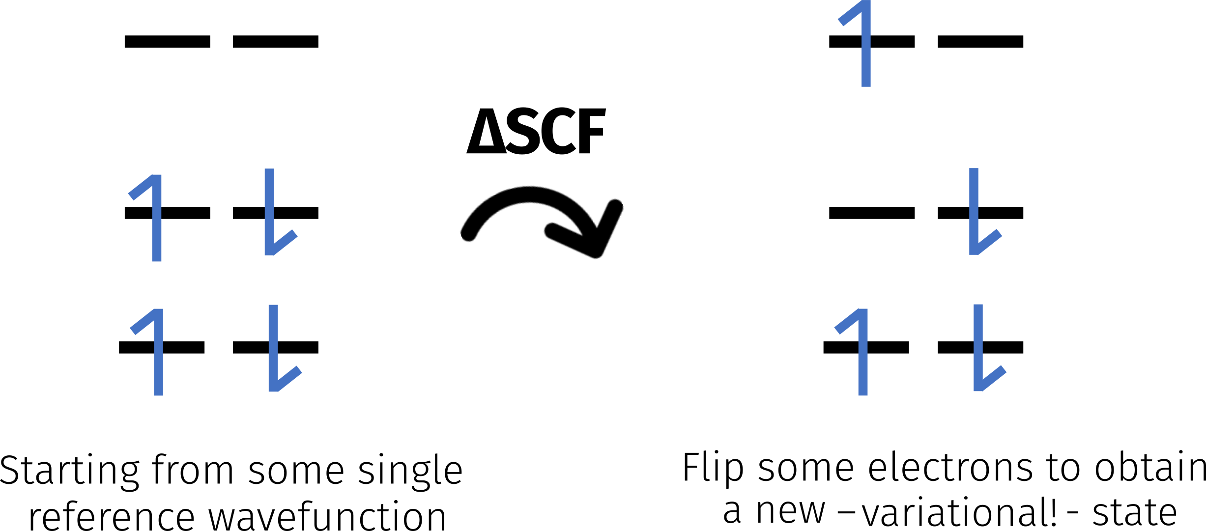
Fig. 5.67 A simple scheme of a HOMO-LUMO excitation state using \(\Delta\)SCF
Using ORCA’s DeltaSCF, we can choose to converge the SCF to a HOMO/LUMO excited state. The
excited state is obtained by fully relaxing the orbitals and can include any contributions such as
the VV10 correlation or CPCM for solvation. Due to the variational optimization of the wave
function, the Hellman-Feynman holds meaning that the gradient on the positions of the nuclei is
available for geometry optimizations, molecular dynamics simulations, reaction path calculations,
and all the other geometry search features ORCA has to offer. Additionally, all properties ORCA can
calculate with a ground state SCF density can be computed with an excited state \(\Delta\)SCF
density as well.
Important
\(\Delta\)SCF states are represented by single-determinant wave functions within a DFT framework. As ground state DFT can struggle with multideterminantal cases, so can excited state DFT. Keep this in mind when tackling such cases!
This description is, for instance, relatively reasonable when
the excited state can be described by a particle-hole interaction. That is for example NOT the case for the HOMO-LUMO excitation of a benzene molecule or most \(\pi\)-\(\pi^{*}\) excited states,
the occupied and virtual orbitals are separated in space such that the relevant exchange integral is zero. Examples include some \(n\)-\(\pi^{*}\) states, long-range charge transfer states etc.,
for closed-shell doubly excited states which can be represented by a single-determinant wavefunction.
Furthermore, \(\Delta\)SCF wave functions can break the symmetries of the Hamiltonian (this is true for ground and excited states). Open-shell singly excited states inherently break the spin symmetry and require spin purification [764].
5.34.1. Theory
In this section, the theory of behind the \(\Delta\)SCF method is discussed.
5.34.1.1. SOSCF L-SR1 method
In \(\Delta\)SCF, one searches a stationary point on the energy surface with respect to the electronic orbital rotation degrees of freedom collected in the orbital rotation matrix
where oo, ov, and vv represent the blocks of \(\boldsymbol{\kappa}\) containing pairwise orbital rotations that mix two occupied, an occupied and a virtual, and two virtual orbitals, respectively. A stationary point is found as
with the energy gradient being
where the right-hand side is a special case of the Baker-Campbell-Hausdorff formula and holds because the space of \(\boldsymbol{\kappa}\) forms the Lie algebra corresponding to the Lie group of its exponential. Since the gradient is always zero for all elements of \(\boldsymbol{\kappa}_{\mathrm{oo}}\) and \(\boldsymbol{\kappa}_{\mathrm{vv}}\), those blocks of \(\boldsymbol{\kappa}\) are dropped as degrees of freedoms in the optimization. As \(e^{\boldsymbol{\kappa}}\) is required to be unitary, \(\boldsymbol{\kappa}\) is required to be anti-Hermitian, dropping several orbital rotations as degrees of freedom in the optimization.
The saddle point search is performed using the L-SR1 quasi-Newton optimizer, which is capable of forming an indefinite model Hessian, starting from an excited state initial guess. To increase the performance of the method and make it more robust, the following standard SOSCF preconditioner is used and allowed to become indefinite as well:
where \(f_{i}\) is the occupation number of orbital \(i\) and \(\epsilon_{i}\) its energy.
5.34.1.2. Generalized Mode Following
The generalized mode following (GMF) method [765, 766] is a more robust but also a bit more expensive saddle point search method that can be used to converge to \(\Delta\)SCF excited state solutions. The method recasts the saddle point search as a minimization by modifying the gradient, such that it corresponds to a modified objective function that has a minimum where the energy function has the target saddle point. Now, a minimization can be performed to locate the target saddle point corresponding to the desired excited state, meaning the robust L-BFGS optimizer can be used instead of the L-SR1 optimizer, the preconditioner can be made positive-definite, and variational collapse to lower-energy solutions other than the targeted one becomes impossible by construction, making MOM unnecessary with GMF. For this to work, the saddle point order \(n\) of the target solution needs to be estimated at the start of the calculation, and the lowest \(n\) eigenpairs of the electronic Hessian need to be evaluated at every electronic optimization step with a finite difference Davidson method.
Once the lowest \(n\) eigenvectors \(v_{i}\) of electronic Hessian are evaluated at each optimization step, the modified gradient is calculated as
5.34.2. Freeze-and-release strategy
In tricky cases, particularly those where the excitation leads to a large amount of charge transfer, it can be advantageous to shift to a freeze-and-release SOSCF strategy [767], which converges the DeltaSCF in two steps:
A constrained optimization freezing all orbitals that are excited, i.e. those orbitals for which the occupation numbers differ from the aufbau occupation. This step reduces to a minimization for the unconstrained orbitals.
An unconstrained optimization as usual.
Step 1 accounts for the orbital relaxation effect due to the first-order change in the electron density after the excitation on the orbitals that are not involved in the excitation. It can be regarded as an elaborate way of generating a very good initial guess for the excited state saddle point search in step 2.
5.34.3. Input and examples
In this section, some example calculations are presented together with the input.
5.34.3.1. First Example: HOMO-LUMO Excited State of Formaldehyde
Let’s begin by trying to converge to the first excited state of formaldehyde and optimize the geometry in that electronic state starting from the regular planar structure:
!PBE DEF2-TZVP OPT FREQ DELTASCF UHF
%SCF ALPHACONF 0,1 END
* XYZ 0 1
C      0.000000    0.000000   -0.602985
O      0.000000    0.000000    0.605394
H      0.000000    0.934673   -1.182175
H      0.000000   -0.934673   -1.182175
*
Besides the regular keywords such as method, basis set, OPT and FREQ, one needs to specify
DELTASCF in the simple input and in this case UHF since the alpha and beta orbitals will be
different due to the single excitation (for doubly-excited states RHF might be sufficient).
It is also necessary to add the ALPHACONF or BETACONF under the %SCF block. That is a minimal
representation of the configuration you want to converge to. In this case, 0,1 means a HOMO/LUMO
transition, where the HOMO has occupation zero and LUMO occupation one. For a HOMO-1/LUMO
transition, it would be ALPHACONF 0,1,1. For a HOMO/LUMO+1 it would be ALPHACONF 0,0,1 and so
on. Just picture what the frontier orbital occupation should look like. Any orbital below the first
zero is assumed to be occupied and any orbital above the last occupied is assumed to be empty.
After the regular startup, the \(\Delta\)SCF-specific print shows:
-------------------------------
DELTA-SCF INITIAL CONFIGURATION
-------------------------------

Alpha: 1.00 1.00 1.00 0.00 1.00 0.00 0.00 0.00
Beta : 1.00 1.00 1.00 1.00 0.00 0.00 0.00 0.00

Hessian update                             ... L-SR1
Aufbau metric                              ... MOM
Keep initial reference                     ... true
Here you can follow the initial configuration and some other important things:
Hessian updaterefers to which method will be used for the SOSCF Hessian update. ORCA’s default isL-BFGS, which forces the electronic Hessian to be positive definite and will always push the system down to a minimum. As we want to go to a saddle point, theL-SR1is set by default forDeltaSCF. More details on Hessian updates and their consequences at this reference from the group of Hannes Jónsson [768].Aufbau metricis the way one measures the “overlap” between the actual and reference wave functions (more details in [761]). It isMOMby default, but can be also set to%SCF PMOM TRUE ENDto usePMOM.Keep initial reference TRUEmeans we will always try to keep the initial reference state defined after the guess phase. That is sometimes calledIMOMin the literature [769]. If%SCF KEEPINITIALREF FALSE ENDis set, it is always the last SCF iteration that is taken as reference.
Important
Here we are using the orbitals of the PMODEL guess because it is trivial. In general, we
recommend always starting the SCF by reading the orbitals of a previously converged ground state
SCF! Please check Restarting SCF Calculations for more info on that.
This calculation trivially converges in 12 steps:
----------------------------------D-I-I-S--------------------------------------------
Iteration    Energy (Eh)       Delta-E    RMSDP     MaxDP     DIISErr  Damp  Time(sec)
-------------------------------------------------------------------------------------
               ***  Starting incremental Fock matrix formation  ***
MOM changed the orbital occupation numbers
  1   -114.2533654537761123     0.00e+00  2.06e-03  6.64e-02  7.14e-02  0.700   0.1
MOM changed the orbital occupation numbers
  2   -114.2675698961360382    -1.42e-02  4.71e-04  1.46e-02  3.08e-02  0.700   0.1
                               ***Turning on AO-DIIS***
MOM changed the orbital occupation numbers
  3   -114.2754325617175226    -7.86e-03  1.98e-04  3.98e-03  2.21e-02  0.700   0.1
MOM changed the orbital occupation numbers
  4   -114.2806616906060100    -5.23e-03  4.98e-04  6.40e-03  1.60e-02  0.000   0.1
MOM changed the orbital occupation numbers
                              *** Initializing SOSCF ***
---------------------------------------S-O-S-C-F-----------------------------------
Iteration   Energy (Eh)           Delta-E    RMSDP     MaxDP    MaxGrad  Time(sec)
-----------------------------------------------------------------------------------
  5    -114.2932665018211225    -1.26e-02  7.19e-05  1.55e-03  2.33e-03     0.1
             *** Restarting incremental Fock matrix formation ***
                          *** Restarting Hessian update ***
  6    -114.2932913947584979    -2.49e-05  5.82e-05  1.33e-03  1.11e-03     0.1
  7    -114.2932671856877818     2.42e-05  2.54e-05  5.00e-04  2.58e-03     0.1
  8    -114.2932914986330530    -2.43e-05  1.76e-05  3.20e-04  1.02e-03     0.1
  9    -114.2932961472105404    -4.65e-06  2.13e-06  6.94e-05  6.42e-05     0.1
 10    -114.2932961779292640    -3.07e-08  2.99e-05  1.10e-03  8.27e-06     0.1
 11    -114.2932921911087050     3.99e-06  3.05e-05  1.12e-03  5.44e-04     0.1
 12    -114.2932961794015654    -3.99e-06  2.45e-08  5.31e-07  2.39e-07     0.1
                *** Gradient check signals convergence ***
Note
The statement MOM changed the orbital occupation numbers is normal, it is just printing what it
is doing. Nothing to worry about.
and one can see from the spin contamination, that this is indeed an open-shell singlet:
----------------------
UHF SPIN CONTAMINATION
----------------------

Warning: in a DFT calculation there is little theoretical justification to
         calculate <S**2> as in Hartree-Fock theory. We will do it anyways
         but you should keep in mind that the values have only limited relevance

Expectation value of <S**2>     :     1.006910
Ideal value S*(S+1) for S=0.0   :     0.000000
Deviation                       :     1.006910
The gradient is then computed, and the geometry is optimized until convergence. Finally the frequencies show this is actually not a minimum, but a saddle point on the geometry space!
-----------------------
VIBRATIONAL FREQUENCIES
-----------------------

Scaling factor for frequencies =  1.000000000  (already applied!)

     0:       0.00 cm**-1
     1:       0.00 cm**-1
     2:       0.00 cm**-1
     3:       0.00 cm**-1
     4:       0.00 cm**-1
     5:       0.00 cm**-1
     6:    -591.31 cm**-1 ***imaginary mode***
     7:     799.56 cm**-1
     8:    1228.37 cm**-1
     9:    1271.29 cm**-1
    10:    2971.77 cm**-1
    11:    3067.96 cm**-1
The reason is: the HOMO/LUMO transition on formaldehyde populates the \(\pi^*\) LUMO, thus breaking the double bound and making the carbon atom pyramidal. If one starts from a slightly distorted structure, it then converges to the actual geometry minimum. Starting from a pyramidal structure:
!wB97M-D4 DEF2-TZVP DELTASCF UHF OPT FREQ
%SCF ALPHACONF 0,1 END
* XYZ 0 1
C          0.00000        0.00000       -0.60298
O         -0.74131       -0.10909        0.45746
H          0.00000        0.93467       -1.18217
H          0.00000       -0.93467       -1.18217
*
now converges to a minimum, as shown by the absence of negative frequencies:
-----------------------
VIBRATIONAL FREQUENCIES
-----------------------

Scaling factor for frequencies =  1.000000000  (already applied!)

     0:       0.00 cm**-1
     1:       0.00 cm**-1
     2:       0.00 cm**-1
     3:       0.00 cm**-1
     4:       0.00 cm**-1
     5:       0.00 cm**-1
     6:     713.25 cm**-1
     7:     826.75 cm**-1
     8:    1206.57 cm**-1
     9:    1292.70 cm**-1
    10:    2826.06 cm**-1
    11:    2893.16 cm**-1
The final geometry is surprisingly accurate for the gas phase formaldehyde, too! We will also show
the results here using the range-corrected, meta-GGA hybrid wB97M-D4 and the double-hybrid DFT
!B2PLYP DEF2-QZVPP AUTOAUX, just to show that MP2 also works.
parameter |
exp. |
PBE |
wB97M-D4 |
B2PLYP |
|---|---|---|---|---|
r(C-O) |
1.323 |
1.300 |
1.310 |
1.311 |
r(C-H) |
1.098 |
1.113 |
1.093 |
1.090 |
\(\angle\)HCH |
118.8 |
115.0 |
117.0 |
116.8 |
\(\angle\)OOP |
34.0 |
41.1 |
36.5 |
37.0 |
exp. taken from [760].
Important
We are using the default ground state SCF algorithm here, AO-DIIS + SOSCF because this is
relatively simple. In general and for more complicated cases, we suggest using the
approximate second-order method, to avoid escaping back to the ground state with !NODIIS NOTRAH,
which is the default for \(\Delta\)SCF.
Important
Do NOT combine \(\Delta\)SCF wavefunctions with CCSD, or any such method with single excitations. It requires a speciallized version of CC which we don’t have yet.
Important
When running the same calculation above with wB97M-D4, there will not be a virtual orbital
between the alpha HOMO-1 and the HOMO (so no negative HOMO-LUMO gap). There is nothing wrong here,
it just optimized the orbitals to the excited state such that the occupation numbers correspond to
an aufbau occupation. Hybrid functionals tend to lower the energy of the occupied orbitals with
respect to the virtual orbitals.
The energy is still higher than the non-\(\Delta\)SCF solution and if you plot the orbitals you will see that the alpha HOMO is now a \(\pi\) orbital instead of an \(n\). The eigenvalues of the electronic Hessian indicate that this solution is a first-order saddle point.
5.34.3.2. Core-ionized States
Another big advantage of the \(\Delta\)SCF is the possibility to converge to core-excited and/or core-ionized states. We have a simple keyword to remove electrons from any orbital, even the deep core ones:
%SCF IONIZEALPHA 2 END
and the electron from orbital number two will be removed. IONIZEBETA works for beta orbitals. One
can start from an anion UHF electronic structure obtained by adding one extra electron and remove a
core electron like this to obtain core-excited states too. Geometry optimization, EPR, and even
TDDFT calculations are all valid for these states.
As an example, the input below will ionize the 1s electron from a water molecule, which corresponds to MO 0 here:
!PBE0 DEF2-TZVP DELTASCF NODIIS UHF
%SCF IONIZEALPHA 0 END
* xyz 0 1
  O      2.127880   -0.361920    0.104770
  H      3.117210   -0.387460    0.070360
  H      1.838520   -0.926280   -0.655730
*
Note
If the orbital is not localized over a single atom, one might need to localized them first!
and one can see from the results that is exactly what it converges to.
----------------
ORBITAL ENERGIES
----------------
                 SPIN UP ORBITALS
  NO   OCC          E(Eh)            E(eV)
   0   0.0000     -20.108086      -547.1688
   1   1.0000      -1.567415       -42.6515
   2   1.0000      -1.057257       -28.7694
   3   1.0000      -0.939315       -25.5601
   4   1.0000      -0.882871       -24.0241
   5   0.0000      -0.304254        -8.2792
   6   0.0000      -0.239285        -6.5113
   7   0.0000       0.044344         1.2066
        (...)
Note
ORCA automatically adjusts charge and multiplicity here. The input should contain those from the reference system!
Here are some examples of binding energies for 1s electrons. The atom from where it was removed is highlighted in bold:
1s ionization |
exp. |
wB97M-V |
|---|---|---|
H2O |
539.82 |
541.17 |
CO2 |
297.69 |
299.10 |
NH3 |
405.56 |
406.82 |
CH3CN |
405.64 |
406.92 |
exp. taken from [770]
5.34.3.3. Diabatic Couplings
\(\Delta\)SCF is also a quite accurate method to obtained diabatic couplings, which can later be used in Markus theory to compute electron transfer rates. These can be computed by calculating the energy difference between electron transfer states and using the Generalized Mulliken-Hush Approach (GMH). For more details please check for example this paper from the group of Blumberger [771].
There is not enough space to go through the details here, but one can get these diabatic coupling from essentially one regular SCF for the ground state + a \(\Delta\)SCF for the excited state. For symmetric systems, this is trivial:
where states \(a\) and \(b\) are diabatic states, and \(\Delta E_{12}\) is the energy difference between adiabatic states \(1\) and \(2\) (which are obtained via SCF solution). Here is an example of the diabatic couplings obtained for a benzene dimer, obtained by starting from the ground state cation and exciting the beta electron with:
%SCF BETACONF 0,1 END
Distance in Ang |
MRCI+Q |
wB97M-V |
TD-DFT |
|---|---|---|---|
3.5 |
435.2 |
473.1 |
593 |
4.0 |
214.3 |
236.7 |
374 |
4.5 |
104.0 |
115.9 |
267.5 |
5.0 |
51.70 |
56.7 |
218.5 |
MRCI+Q taken from [771]
5.34.3.4. Generalized Mode Following
For an example GMF calculation, we return to the formaldehyde molecule, this time targeting a
HOMO-LUMO+1 excitation to keep it interesting and add the simple input keyword GMF:
!WB97X-D4 DEF2-SVP UKS DELTASCF GMF
%SCF ALPHACONF 0,0,1 END
* XYZ 0 1
O         -3.54418        1.61112        0.04891
C         -4.12047        0.61074       -0.35955
H         -3.36418       -0.41948       -0.79627
H         -4.84699        0.73407       -1.42962
*
If not provided in the input, the target saddle point order is estimated either by using the orbital
energies or by
evaluating the number of negative eigenvalues of the electronic Hessian. In the former case, the
target saddle point order is approximated as the number of pairs of an occupied and a virtual
orbital where the occupied orbital has a larger energy than the virtual orbital at the excited state
initial guess after the excitation has been performed. In our example, this yields a saddle point
order of 2, as is estimated by default and printed together with some other default input parameters
in the DeltaSCF block:
-------------------------------
DELTA-SCF INITIAL CONFIGURATION
-------------------------------

Alpha: 1.00 1.00 1.00 0.00 0.00 1.00 0.00 0.00 0.00
Beta : 1.00 1.00 1.00 1.00 0.00 0.00 0.00 0.00 0.00

Hessian update                             ... L-BFGS/GMF
Generalized mode following:
 Target saddle point order                 ... 2
 Finite difference generalized Davidson method:
  Finite difference mode                   ... Forward
  Finite difference step size              ... 1.000e-03
  Max. size of Krylov subspace             ... 20
  Convergence tolerance                    ... 1.000e-02
  Max. number of iterations                ... 100
Aufbau metric                              ... Fixed occupations
Before every optimization step, the lowest 2 (same as target saddle point order) eigenpairs of the electronic Hessian are evaluated, and once converged below the tolerance, the eigenvalues are printed, e.g. for the first optimization step:
Solving for 2 Hessian eigenvectors
    It.    Root MAX Err.:          1          2
    1                      6.520e-02  6.276e-02
    2                      3.193e-02  2.817e-02
    3                      1.511e-02  9.423e-03
    4                      3.889e-03  9.417e-03
    Eigenvalues:          -3.316e-01 -2.404e-01
After a few optimization steps, the evaluation of the Hessian eigenpairs requires no further adjustments, so that the Davidson runs converge immediately:
        Solving for 2 Hessian eigenvectors
            It.    Root MAX Err.:          1          2
            1                      5.165e-03  8.433e-03
            Eigenvalues:          -2.574e-01 -1.792e-01
   11    -114.1023998750192305    -1.06e-05  1.06e-03  1.96e-02  5.46e-04     1.3
        Solving for 2 Hessian eigenvectors
            It.    Root MAX Err.:          1          2
            1                      5.755e-03  8.231e-03
            Eigenvalues:          -2.575e-01 -1.791e-01
   12    -114.1024101850037624    -1.03e-05  6.43e-04  1.25e-02  3.11e-04     1.3
        Solving for 2 Hessian eigenvectors
            It.    Root MAX Err.:          1          2
            1                      6.190e-03  8.354e-03
            Eigenvalues:          -2.575e-01 -1.790e-01
   13    -114.1024129524389963    -2.77e-06  3.67e-04  7.30e-03  2.00e-04     1.3
        Solving for 2 Hessian eigenvectors
            It.    Root MAX Err.:          1          2
            1                      6.264e-03  8.286e-03
            Eigenvalues:          -2.574e-01 -1.790e-01
   14    -114.1024142211099530    -1.27e-06  8.68e-05  1.34e-03  1.46e-04     1.3
        Solving for 2 Hessian eigenvectors
            It.    Root MAX Err.:          1          2
            1                      6.396e-03  8.439e-03
            Eigenvalues:          -2.574e-01 -1.790e-01
   15    -114.1024145538739987    -3.33e-07  4.56e-05  7.31e-04  9.17e-05     1.3
                 **** Energy Check signals convergence ****
In this simple example, one would expect the configuration to be conserved during the optimization. This is not the case here, again, because a hybrid functional is used. The occupied orbitals are stabilized with respect to the virtual ones leading to this configuration:
----------------
ORBITAL ENERGIES
----------------
                 SPIN UP ORBITALS
  NO   OCC          E(Eh)            E(eV)
   0   1.0000     -19.374322      -527.2021
   1   1.0000     -10.431285      -283.8497
   2   1.0000      -1.258409       -34.2430
   3   1.0000      -0.755807       -20.5666
   4   1.0000      -0.635639       -17.2966
   5   1.0000      -0.591213       -16.0877
   6   1.0000      -0.584445       -15.9036
   7   0.0000      -0.143277        -3.8988
   8   1.0000      -0.113247        -3.0816
   9   0.0000      -0.061224        -1.6660
  10   0.0000       0.146574         3.9885
  11   0.0000       0.251438         6.8420
  12   0.0000       0.490702        13.3527
  13   0.0000       0.537161        14.6169
  14   0.0000       0.565655        15.3923
  15   0.0000       0.624632        16.9971
  16   0.0000       0.649717        17.6797
  17   0.0000       0.710983        19.3468
  18   0.0000       0.928559        25.2674
The two lowest eigenvalues of the Hessian at the last optimization step are clearly negative, so this solution is a second-order saddle point, as expected and targeted in the optimization. Do not rely on the configuration to determine the saddle point order if you use hybrid functionals!
5.34.3.5. Freeze-and-release strategy
Let’s take a look at a tricky excited state of the 90-degrees-twisted N-phenylpyrrole molecule.
We first perform a ground state SCF calculation without DeltaSCF using this input:
!UKS aug-cc-pVDZ PBE

*xyz 0 1
C       10.13954933      10.09711395      12.38421108
C       11.34646202      10.09711395      13.07460199
C        8.93263664      10.09711395      13.07460199
C       10.13954933      10.09711395      15.16101197
C       11.34465495      10.09711395      14.46510328
C        8.93444370      10.09711395      14.46510328
C       10.13954933      11.21630306      10.16939448
C       10.13954933       8.97792484      10.16939448
C       10.13954933      10.80761594       8.85675649
C       10.13954933       9.38661196       8.85675649
N       10.13954933      10.09711395      10.96513494
H       12.26979504      10.09711395      12.51888639
H        8.00930362      10.09711395      12.51888639
H       12.27909865      10.09711395      15.00190089
H        8.00000000      10.09711395      15.00190089
H       10.13954933      10.09711395      16.23847837
H       10.13954933      12.19422790      10.60962753
H       10.13954933       8.00000000      10.60962753
H       10.13954933      11.45309491       8.00000000
H       10.13954933       8.74113299       8.00000000
*
This calculation yields an energy of -440.702 E\(_\mathrm{h}\) and a dipole moment of 2.181 D. Now we
perform an excited state calculation with DeltaSCF starting from this converged ground state
solution and exciting an electron from the HOMO to the LUMO in the alpha spin channel with this
input:
!UKS aug-cc-pVDZ PBE DeltaSCF
!SOSCF NoDIIS NoTRAH
!MORead
!SCFCheckGrad

%moinp "gs.gbw"

%scf
AlphaConf 0,1
DoMOM false
SOSCFMaxStep 0.1
end

*xyz 0 1
C       10.13954933      10.09711395      12.38421108
C       11.34646202      10.09711395      13.07460199
C        8.93263664      10.09711395      13.07460199
C       10.13954933      10.09711395      15.16101197
C       11.34465495      10.09711395      14.46510328
C        8.93444370      10.09711395      14.46510328
C       10.13954933      11.21630306      10.16939448
C       10.13954933       8.97792484      10.16939448
C       10.13954933      10.80761594       8.85675649
C       10.13954933       9.38661196       8.85675649
N       10.13954933      10.09711395      10.96513494
H       12.26979504      10.09711395      12.51888639
H        8.00930362      10.09711395      12.51888639
H       12.27909865      10.09711395      15.00190089
H        8.00000000      10.09711395      15.00190089
H       10.13954933      10.09711395      16.23847837
H       10.13954933      12.19422790      10.60962753
H       10.13954933       8.00000000      10.60962753
H       10.13954933      11.45309491       8.00000000
H       10.13954933       8.74113299       8.00000000
*
This simple-seeming excitation leads to a large charge transfer from the phenyl group to the
pyrrole group which makes this excited state tricky to converge. To this end, we reduce the maximum
step size of the SOSCF optimization from 0.2 (default) to 0.1 with SOSCFMaxStep 0.1 and deactivate
MOM with DoMOM false since MOM tends to become counterproductive for cases with heavy charge
transfer. We also use only SOSCF and deactivate DIIS and TRAH using the simple input
!SOSCF NoDIIS NoTRAH and force a convergence check for the SOSCF gradient with !SCFCheckGrad.
The latter amounts to personal preference.
This calculation converges to a solution with an excitation energy of 189 mE\(_{\mathrm{h}}\) and a dipole moment difference to the ground state of 4.958 D, which are both smaller than expected for this heavy charge transfer state. This is known as a variational collapse, i.e. the calculation converged to a lower-energy solution than desired.
To counteract this variational collapse, we use the freeze-and-release SOSCF approach by adding
FreezeAndRelease (or FRSOSCF) to the simple input line:
!UKS aug-cc-pVDZ PBE DeltaSCF FreezeAndRelease
!MORead
!SCFCheckGrad

%moinp "gs.gbw"

%scf
AlphaConf 0,1
DoMOM 0
SOSCFConvFactor 500
SOSCFMaxStep 0.1
end

*xyz 0 1
C       10.13954933      10.09711395      12.38421108
C       11.34646202      10.09711395      13.07460199
C        8.93263664      10.09711395      13.07460199
C       10.13954933      10.09711395      15.16101197
C       11.34465495      10.09711395      14.46510328
C        8.93444370      10.09711395      14.46510328
C       10.13954933      11.21630306      10.16939448
C       10.13954933       8.97792484      10.16939448
C       10.13954933      10.80761594       8.85675649
C       10.13954933       9.38661196       8.85675649
N       10.13954933      10.09711395      10.96513494
H       12.26979504      10.09711395      12.51888639
H        8.00930362      10.09711395      12.51888639
H       12.27909865      10.09711395      15.00190089
H        8.00000000      10.09711395      15.00190089
H       10.13954933      10.09711395      16.23847837
H       10.13954933      12.19422790      10.60962753
H       10.13954933       8.00000000      10.60962753
H       10.13954933      11.45309491       8.00000000
H       10.13954933       8.74113299       8.00000000
*
FreezeAndRelease only works for SOSCF, so SOSCF, NoDIIS, and NoTRAH are implicite and do not
need to be specified. We also apply a factor of 500 that the convergence criteria of the constrained
minimization are multiplied by since the constrained minimization does not need to be converged as
tightly as the subsequent unconstrained optimization. This strategy saves some iterations in the
constrained part of the calculation without compromising the final result.
This strategy yields an excitation energy of 194 mE\(_{\mathrm{h}}\), a bit higher than the previous one, and a dipole moment difference to the ground state of 9.669 D. This is the desired result.
Typically, the freeze-and-release approach takes a few more iterations than the regular SOSCF, but it avoids variational collapse much more reliably. In the presented case, the regular SOSCF converges in a total of 38 energy/gradient evaluations, while the freeze-and-release strategy takes only 21 energy/gradient evaluations.
Note
The statement Scaled step length from x to 0.100000 is indicating that a relatively large step
was about to be taken. Scaling it down typically results in more robust but less efficient
convergence. It can be adjusted to the challenges of the system under investigation.
The freeze-and-release strategy can be combine with GMF yielding an even more robust strategy. In this case, the target saddle point order is estimated at the solution of the constrained minimization step since the quality of the estimate increases then. For hybrid functionals, the default estimate is obtained in the first Davidson run. Otherwise, the orbital energies are used.
5.34.4. Full keyword list
The simple input keywords related to \(\Delta\)SCF are collected in tab. Table 5.26.
Keyword |
Description |
|---|---|
|
Activates \(\Delta\)SCF |
|
Activates freeze-and-release strategy |
|
Activates generalized mode following |
|
Sets SOSCF quasi-Newton method to L-BFGS |
|
Sets SOSCF quasi-Newton method to L-SR1 |
The input keywords of the %SCF block related to \(\Delta\)SCF are collected in tab.
Table 5.27.
Keyword |
Options |
Description |
|---|---|---|
|
|
Maximum step size |
|
|
Start DeltaSCF from an input converged ground state solution or assume it is an excited state solution? |
|
|
Perform a diagonalization of the occupied and virtual orbital blocks of the Fock matrix at the start? |
|
|
Use the maximum overlap method? |
|
|
Always keep initial reference: IMOM? |
|
|
Use the PMOM metric instead of the regular MOM? |
|
Define the occupation of the frontier orbitals in alpha and beta spin channels |
|
|
HOMO\(\rightarrow\)LUMO excitation |
|
|
HOMO\(\rightarrow\)LUMO+1 excitation |
|
|
HOMO-1\(\rightarrow\)LUMO excitation |
|
|
Double HOMO\(\rightarrow\)LUMO excitation (only valid for |
|
|
|
Remove electron from specified MOs in alpha and beta spin channel |
|
SOSCF quasi-Newton method for Hessian update |
|
|
Limited-memory symmetric rank-1 update |
|
|
Limited-memory Broyden-Fletcher-Goldfarb-Shanno update |
|
|
Limited-memory Powell update |
|
|
Limited-memory Bofill update, a combination of L-SR1 and L-Powell |
|
|
|
Activate freeze-and-release SOSCF? |
|
|
Maximum step size for the constrained minimization |
|
|
Factor to multiply convergence criteria with in the constrained minimization. E.g. 100 loosens the criteria by two orders of magnitude |
|
Hessian update for constrained minimization |
|
|
Limited-memory symmetric rank-1 update |
|
|
Limited-memory Broyden-Fletcher-Goldfarb-Shanno update |
|
|
Limited-memory Powell update |
|
|
Limited-memory Bofill update, a combination of L-SR1 and L-Powell |
|
|
|
Write a GBW file for the constrained solution |
|
|
Use generalized mode following? |
|
|
Maximum number of Davidson iterations |
|
|
Davidson convergence tolerance for the maximum component of each residual vector |
|
|
Davidson maximum size of the Krylov subspace per target eigenvector, meaning this will be multiplied by the target saddle point order |
|
Davidson finite difference stencil to use |
|
|
One displaced gradient evaluation, linear accuracy in finite difference step size |
|
|
Two displaced gradient evaluations, quadratic accuracy in finite difference step size |
|
|
|
Davidson finite difference step size |
|
|
GMF Optional user-defined target saddle point order |
|
GMF Target saddle point order estimate |
|
|
Let the algorithm determine what is best |
|
|
Use the excitation configuration |
|
|
Use the diagonal Hessian approximation (only different from |
|
|
Use number of negative eigenvalues in first Davidson run (targets more eigenpairs in first run) |
|
|
|
GMF only: Update the SPO with the number of negative eigenvalues of the first Davidson run? |
|
|
How many eigenvectors of the Hessian to target more for the SPO estimate |
|
|
Only eigenvalues below this threshold are considered negative enough for the SPO estimate |
|
SOSCF preconditioner to use |
|
|
Regular preconditioner based on the orbital energy differences |
|
|
|
|
|
GMF only: Mixes preconditioner with a gradient expansion (ration given by |
|
|
|
Mixing factor for |