5.3. Fractional Occupation Number Weighted Density (FOD)

Many approximate QC methods do not yield reliable results for systems with significant static electron correlation (SEC) and moreover it is often difficult to predict if the system in question suffers from SEC or not. Existing scalar SEC diagnostics (e.g., the $T_1$ diagnostic) do not provide any information where the SEC is located in the molecule. Furthermore, often quite expensive calculations have to be performed first (e.g., CCSD) in order to judge the reliability of the results based on a single value. Molecular systems with strong SEC (e.g. covalent bond-breaking, biradicals, open-shell transition metal complexes) are usually characterized by small energy gaps between frontier orbitals, and hence, the existence of many equally important determinants in their electronic wavefunction. This finding is used in the fractional occupation number weighted density (FOD) analysis proposed by Hansen and Grimme.[588] The FOD analysis is based on finite temperature KS-DFT where the fractional occupation numbers are determined from the Fermi distribution (“Fermi smearing”).

(5.25)$$f_i=\frac{1}{e^{({\epsilon }_i-E_F)/k{T}_{el}}+1}$$

The central quantity of the FOD analysis is the fractional occupation number weighted electron density (${\rho }^{FOD}$), a real-space function of the position vector $r$:

(5.26)$${\rho }^{FOD}(r)=\sum _i^N({\delta }_1-{\delta }_2{f}_i)|{\phi }_i(r){|}^2$$

(${\delta }_1$ and ${\delta }_2$ are unity if the level is lower than $E_F$ while they are 0 and $-1$, respectively, for levels higher than $E_F$). The $f_i$ represent the fractional occupation numbers (0$\le f_i\le$1; sum over all electronic single-particle levels obtained by solving self-consistently the KS-SCF equations minimizing the free-electronic energy).

${\rho }^{FOD}(r)$ can be plotted using a pre-defined contour surface value (see Section FOD Plots). The integration of ${\rho }^{FOD}$ over all space yields as additional information a single size-extensive number termed $N_{FOD}$ which correlates well with other scalar SEC diagnostics and can be used to globally quantify SEC effects in the molecule. Accordingly, FOD analysis and plots represent a cost-effective and robust way to identify the ‘hot’ (strongly correlated) electrons in a molecule and to choose appropriate approximate quantum chemical methods for a subsequent computational study of the systems in question. Based on our experience, the following rules of thumb can be derived:

• no significant ${\rho }^{FOD}$: use (double)-hybrid functionals or (DLPNO-)CCSD(T) (single-reference electronic structure)

• significant but rather localized ${\rho }^{FOD}$: use semi-local GGA functionals (or hybrid functional with low Fock-exchange, avoid HF or MP2; slight multi-reference character)

• significant and delocalized ${\rho }^{FOD}$: use multi-reference methods (or finite temperature DFT; strong multi-reference character)

Warning

Even though the FOD is intuitive and easy-to-use, it is not a 100% safe diagnostic for MR character and should only be used as a first indication. We recommend to always combine the FOD analysis with more sophisticated multi-reference diagnostics.

Tip

Mulliken reduced orbital charges based on ${\rho }^{FOD}(r)$ (see Mulliken Population Analysis) offer a fast alternative to get the information of the FOD plot (cf. Example: p-Benzyne).

5.3.1. Basic Usage

The FOD analysis is a very efficient and practicable tool to get information about the amount and localization of SEC in the system of question and can be invoked via the !FOD simple input keyword.

! FOD

This will perform the analysis at the default TPSS/def2-TZVP (TightSCF) level that was chosen since it is fast and robust. Besides the standard analysis output (cf. Section 5.3.3), ${\rho }^{FOD}$ is stored in the file basename.scfp_fod file which is included in the general basename.densities container (for plotting the FOD, see Section 5.3.2).

The FOD analysis can be customized via simple input and the %scf block.

! B3LYP def2-TZVP TightSCF

%scf
 SmearTemp 9000
end

Important

• ${\rho }^{FOD}$ (and $N_{FOD}$) strongly depend on the orbital energy gap which itself depends almost linearly on the amount of the non-local Fock exchange admixture $a_x$ (cf. hybrid DFT). The following (empirical) function of the optimal electronic temperature $T_{el}$ on $a_x$

  (5.27)$$T_{el}=20000\text{K}\times a_x+5000\text{K}$$

  is used to ensure that similar results of the FOD analysis are obtained with various functionals. For example, the SmearTemp has to be 5000 K for TPSS ($a_x$ = 0), 9000 K for B3LYP ($a_x$ = 20%), 10000 K for PBE0 ($a_x$ = 25%), and 15800 K for M06-2x ($a_x$ = 54%).

Some Notes on FOD

• The FOD analysis is not strongly dependent on the employed basis set (see supplementary information of the original publication[588]).

• The FOD analysis will be always printed (including Mulliken reduced orbital charges based on ${\rho }^{FOD}$) if SmearTemp $>$ 0 K.

• Since the ${\hat{S}}^2$ expectation value is not defined for fractional occupation numbers, its printout is omitted.

• The FOD analysis may also be useful for finding a suitable active space for e.g. in CASSCF calculations.

5.3.2. FOD Plots

The fractional occupation number weighted electron density (${\rho }^{FOD}$, see Fractional Occupation Number Weighted Density (FOD)) can be plotted in 3D for a pre-defined contour surface value which, after extensive testing, was set to the default value of $\sigma =0.005$ e/Bohr${}^3$. In order to allow comparison of various systems this value should be kept fix (in critical cases, one may also check the FOD plot with a a smaller value of $\sigma =0.002$ e/Bohr${}^3$ for comparison). The FOD is strictly positive in all space and resembles orbital densities (e.g., $\pi$-shape in large polyenes) or the total charge density for an ideal ‘metal’ with complete orbital degeneracy in simple cases.

Basically, ${\rho }^{FOD}$ can be plotted analogously to an electron density using the orca_plot utility program and the generated basename.scfp_fod density file that is stored in the basename.scfp_fod is stored in the basename.densities container.

To do so call orca_plot in interactive mode via

orca_plot basename.gbw -i

The interface will now show various plot options.

PlotType       ... MO-PLOT
MO/Operator    ... 0 0
Output file    ... (null)
Format         ... Grid3D/Binary
Resolution     ... 40 40 40
Boundaries     ...   -22.359392    16.311484 (x direction)
                     -12.628859    13.574504 (y direction)
                      -7.001812     7.002006 (z direction)

       1 - Enter type of plot
       2 - Enter no of orbital to plot
       3 - Enter operator of orbital (0=alpha,1=beta)
       4 - Enter number of grid intervals
       5 - Select output file format
       6 - Plot CIS/TD-DFT difference densities
       7 - Plot CIS/TD-DFT transition densities
       8 - Set AO(=1) vs MO(=0) to plot
       9 - List all available densities
      10 - Perform Density Algebraic Operations

      11 - Generate the plot
      12 - exit this program
Enter a number: 

To check all available densities in the basename.densities container one can use the 9 - List all available densities option.

---------------------
List of density names
---------------------

Index:                               Name of Density
----------------------------------------------------
    0:                             basename.scfp_fod   <--- required for FOD plot
    1:                                 basename.scfp
    2:                                 basename.scfr

The most general way to create the FOD plot is now to create a .cube file that can be visualized with many external programs like ChimeraX or Chemcraft (cf. Graphical User Interfaces).

To do so we use the following subsequent user inputs to orca_plot:

1 (type of plot)
2 (electron density)
n (default name: no)
basename.scfp_fod (name of the FOD file)
4 (number of grid intervals)
120 (NGrid)
5 (output file format)
7 (cube)
10 (generate plot)
11 (exit)

Warning

Note that producing .cube files can become very large and their generation with orca_plot may take a considerable amount of time for larger molecules. This is particularly the case if high quality plots using tight grid resolution settings (i.e., 120x120x120 resolution) are used for publication purposes.

It is also possible to generate *.cube files from ${\rho }^{FOD}$ (analogously to electron density plots) with other programs that can read ORCA’s baseame.gbw and electron density files by simply using the basename.scfp_fod file instead of the basename.scfp file.

An example FOD plot for Ni(bis-dithiolene) is shown below (Fig. 5.2). It was generated with ChimeraX and a .cube file generated by orca_plot and clearly shows the strong FOD on the metal center and the adjacent ligands. This observation is in line with various studies on the multi-reference character of this complex.

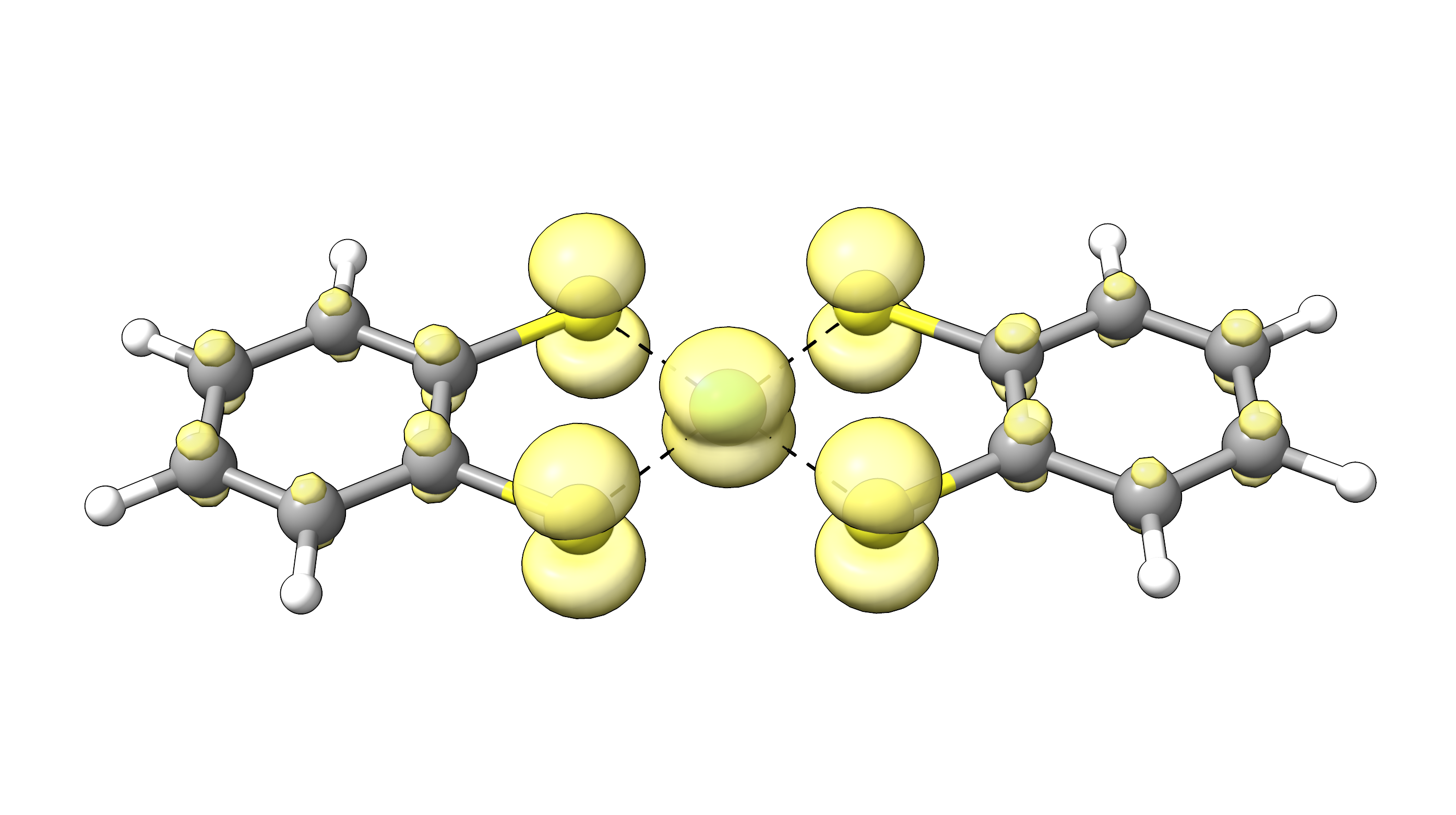
Fig. 5.2 FOD plot at $\sigma =0.005$ e/Bohr${}^3$ (TPSS/def2-TZVP (T = 5000 K) level) for the NiBDT complex (FOD depicted in yellow).

More examples of FOD plots generated with the same setup can be found in the original publication and corresponding supplementary information.[588]

5.3.3. Example: p-Benzyne

In this example, the FOD analysis for the ground state of p-Benzyne is performed.

! FOD 

* xyz 0 1
C 0.0000000  1.2077612  0.7161013
C 0.0000000  0.0000000  1.3596219
C 0.0000000 -1.2077612  0.7161013
C 0.0000000 -1.2077612 -0.7161013
C 0.0000000  0.0000000 -1.3596219
C 0.0000000  1.2077612 -0.7161013
H 0.0000000  2.1606260  1.2276695
H 0.0000000 -2.1606260  1.2276695
H 0.0000000 -2.1606260 -1.2276695
H 0.0000000  2.1606260 -1.2276695
*

The respective output reads:

-------------------------------------------------------------------------------------------
                                      ORCA LEAN-SCF
                              memory conserving SCF solver
-------------------------------------------------------------------------------------------

----------------------------------------D-I-I-S--------------------------------------------
Iteration    Energy (Eh)           Delta-E    RMSDP     MaxDP     DIISErr   Damp  Time(sec)
-------------------------------------------------------------------------------------------
               ***  Starting incremental Fock matrix formation  ***
    1    -230.8982516003082139     0.00e+00  5.01e-03  1.01e-01  1.12e-01  0.700   1.7
Warning: op=0 Small HOMO/LUMO gap (  -0.021) - skipping pre-diagonalization
         Will do a full diagonalization
    2    -230.9463607195993120    -4.81e-02  1.15e-03  2.59e-02  4.06e-02  0.700   1.6
                               ***Turning on AO-DIIS***
  ... etc.
   12    -231.0033984839932089    -5.02e-09  3.33e-07  7.37e-06  7.95e-06  0.000   1.1
                 **** Energy Check signals convergence ****

FOD:
 Fermi smearing:E(HOMO(Eh)) = -0.201252 MUE = -0.179318 gap=   1.119 eV

 N_FOD =  0.920364

The high $N_{FOD}$ already indicates strong SEC and checking the Mulliken reduced orbital charges based on ${\rho }^{FOD}(r)$ (see Mulliken Population Analysis) gives a first impression about the localization of hot electrons in the molecule. The printout for the first carbon atom is given below:

------------------------------------------
FOD BASED MULLIKEN REDUCED ORBITAL CHARGES
------------------------------------------
  0 C s       :     0.006371  s :     0.006371
      pz      :     0.016375  p :     0.030785
      px      :     0.009893
      py      :     0.004516
      dz2     :     0.004248  d :     0.010308
      dxz     :     0.000254
      dyz     :     0.004855
      dx2y2   :     0.000860
      dxy     :     0.000091
      f0      :     0.000006  f :     0.000378
      f+1     :     0.000014
      f-1     :     0.000309
      f+2     :     0.000002
      f-2     :     0.000006
      f+3     :     0.000010
      f-3     :     0.000032

If other population analysis printouts are wanted the user is referred to the Löwdin analysis (Löwdin Population Analysis) which is turned on by default using the total SCF density of the calculation, also in the case of finite electronic temperature.

The plot the ${\rho }^{FOD}$ for p-Benzyne clearly shows the significant and rather delocalized FOD (${}^1{A}_g$), thus indicating that multi-reference methods would be needed for reliable computational study of this molecule.

Fig. 5.3 FOD plot at $\sigma =0.005$ e/Bohr${}^3$ (TPSS/def2-TZVP (T = 5000 K) level) for the ${}^1{A}_g$ ground state of $p$-benzyne (FOD depicted in yellow).