6.1. Overview on ORCA’s Multiscale Implementation
ORCA features five primary methods suitable for diverse applications such as proteins, DNA, large molecules, explicit solvation, and crystalline solids:
Additive QM/MM for proteins and DNA/RNA.
QM1/QM2 (2-layered ONIOM) for small proteins, RNA, large molecules and explicit solvation.
QM1/QM2/MM (3-layered ONIOM) for proteins and DNA/RNA.
MOL-CRYSTAL-QMMM for molecular crystals.
IONIC-CRYSTAL-QMMM for semiconductors and insulators.
All methods integrate seamlessly with other ORCA modules, simplifying the preparation and execution of multiscale calculations.
The multiscale features are optimally connected to all other modules and tools available in ORCA allowing the user to handle multiscale calculations from a QM-centric perspective in a simple and efficient way, with a focus on simplifying the process to prepare, set up and run multiscale calculations. Since version 6.1 ORCA provides an automated tool for setting up QM and active regions, which is described here.
From the input side all methods share a common set of concepts and keywords, which will be outlined in this section. In subsequent sections the different methods are described and further input options are discussed.
6.1.1. Combining Multiscale Features with other ORCA Features
The multiscale features can be used together with all other possible ORCA methods:
Single Point Calculations: Use all kinds of available electronic structure methods as QM method.
Optimization: Use all kinds of geometry optimizations with all kinds of constraints, TS optimization, relaxed surface scans, and the ScanTS feature. Use the L-Opt and L-OptH features including the combination of all kinds of fragment optimizations (fix fragments, relax fragments, relax only specific elements in fragments, treat a fragment as a rigid body).
Transition States and Minimum Energy Paths: Use all kinds of Nudged-Elastic Band calculations Nudged-Elastic Band calculations (Fast-NEB-TS, NEB, NEB-CI, NEB-TS, including their ZOOM variants) and Intrinsic Reaction Coordinate calculations. (not implemented for
MOL-CRYSTAL-QMMMandIONIC-CRYSTAL-QMMM)Conformational Searches: Conformational Searches can be run with ORCA’s GOAT module.
Frequency Calculations: Use regular frequency calculations. If required, ORCA automatically switches on the Partial Hessian Vibrational Analysis (PHVA) [528] calculation. (not tested for
IONIC-CRYSTAL-QMMM)Molecular Dynamics: Use the Molecular Dynamics (MD) module for Born-Oppenheimer MD (BOMD) with QM/MM in combination with all kinds of electronic structure methods. (not implemented for
MOL-CRYSTAL-QMMMandIONIC-CRYSTAL-QMMM)Property Calculation: All kinds of regular property calculations are available. For electrostatic embedding the electron density is automatically perturbed by the surrounding point charges.
Excited State Calculations: Use all kinds of excited state calculations (TD-DFT, EOM, single point calculations, optimizations, frequencies).
6.1.2. Required Settings for a Multiscale Simulation
In the following, the basic concepts are introduced.
QM atoms: The user can define the QM region either directly, or via flags in a pdb file. See QM and Active Region Definition. For an automated buildup
of the QM region with miminal user input see here.
Active Atoms: The user can choose an active region, e.g. for geometry optimizations the atoms that are optimized, for a frequency calculation the atoms that are allowed to vibrate for the PHVA, or for an MD run the atoms that are propagated. More background is provided here. Input options on how to define the active region in an automated way or in an explicit way are provided below.
A minimal user input for an ONIOM2 type calculation looks like this.
!QM/XTB
%qmmm
  QMCoreAtoms {7 12} end
  ActiveCoreAtoms {7 12} end
end
*xyz 0 1
...
Other aspects that often need to be addressed for multiscale simulations are treated automatically and with reasonable defaults- which can, of course, be controlled by the user. The boundary treatment, i.e. bonds that have to be cut between QM and MM region, and the treatment of overpolarization is covered in the paragraph Boundary Region. Available embedding types are discussed in section Embedding Types. QM2 atoms, which define the low-level region in 3-layer ONIOM calculations, are discussed in section QM2 Atoms.
Detailed information on the different available input and runtime options and additionally available keywords (see Additional Keywords) are given below.
Note
In order to check the multiscale setup done by ORCA, without the need to run the entire simulation, you can
invoke the keyword ! QMMMSetup.
This makes sure that ORCA stops after the multiscale preparation. The information on the QMMM setup is
printed in the output, and
a file with the QM region including link atoms is stored (basename_QM.xyz).
6.1.3. QM and Active Region Definition
QM and active region atoms can be defined in three different ways:
Explicit definition of all atom indices.
Defining the most important atoms (the
coreatoms) and ORCA determines the full QM and active region.Definition in a pdb file.
6.1.3.1. Explicit Definition of QM and Active Region
The QM and active region can be directly defined in the input as shown in the following example:
%qmmm
 QMAtoms {0 1 2 27 28} end      # lists of atoms (counting starts from 0) or
 ActiveAtoms {0:5 16 21:30} end # ranges of atoms (range defined via start:end)
end
*pdbfile 0 1 ubq.pdb
6.1.3.2. Automated Definition of QM and Active Region
A standard approach in the QMMM scientific literature for defining QM and active regions involves:
6.1.3.2.1. Identifying Important Atoms or Functional Groups
Examples include:
Atoms involved directly in bond formation or breakage.
Functional groups essential for spectroscopy.
Metal ions central to catalytic activities.
Entire molecules or ligands binding to proteins.
Additional criteria as necessary.
6.1.3.2.2. Including Surrounding Atoms
Include all atoms within a defined spatial distance around these important atoms.
6.1.3.2.3. Applying Rules to Avoid Artifacts
Specifically ensure that:
The boundary between QM and MM regions cuts through a non-polarized single bond.
The topological distance between two QM-MM cuts (the MM gap) is sufficiently large,
preventing overly close placement of link atoms.
6.1.3.2.4. Automated procedure in ORCA 6.1
In ORCA 6.1, an automatic scheme has been developed to manage this multistep process. Users specify only key atoms (core atoms) that define the core part of the QM and active regions.
ORCA requires:
Knowledge of the system’s topology.
Information about functional groups within the system.
Using the newly introduced fragmentation procedure, ORCA automatically determines this information at the start of the calculation. Functional groups are stored as separate fragments based on the user-selected fragmentation procedure.
6.1.3.2.5. Steps of the Automated Procedure (Illustrated for QM Region; analogous steps apply for active regions)
Accept user-defined input
QMCoreAtoms.If
QMCore_TypeisFragments, extendQMCoreAtomsto entire fragments, producing an updatedQMCoreAtomsset.Determine all atoms within
QMCore_ExtensionÅ aroundQMCoreAtoms, yieldingQMAtoms.If
QMCoreExtension_TypeisFragments, extendQMAtomsto entire fragments, updating the set again.Include any explicitly user-defined atoms (
QMAtoms) in the automatically generated set.If
CheckAutoFragForQMGapsistrue, verify no topologically close QM atoms are separated by fewer MM atoms thanQMGap_MinLength. If so, add necessary connecting fragments toQMAtoms.If
CheckAutoFragBoundariesistrue, ensure that QM-MM boundaries do not cut polarized or problematic bonds.Repeat steps 6 and 7 until no further fragments need addition.
Note
You can add the keyword QMMMSetup to your input. This allows you to check the autogenerated QM region (basename_QM.xyz) and verify the charge and multiplicity required for the actual multiscale calculation.
that is needed for the actual multiscale calculation.
The automated QM and active region setup can be defined in the input as shown in the following example:
! QM/XTB
! QMMMSetup # just do the preparation and stop
%qmmm
 QMCoreAtoms {2032} end
 ActiveCoreAtoms {2032} end
 frag
   FragProc NABackbone, NASideChains, FunctionalGroups, Extend, Connectivity
 end
end

*xyz 0 1
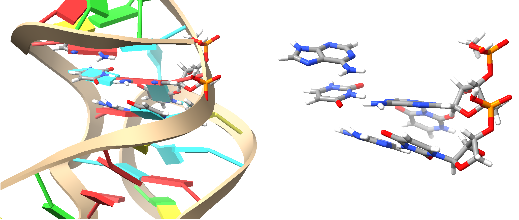
Fig. 6.1 QM region for QMCoreAtom 2032. Left is the QM region in ball-and-stick style as part of the full system in cartoon style, right is the QM region with link atoms.
In the above example, which is a ligand bound to RNA, we first define the fragments using the fragmentator) using RNA specific groups and functional groups (for the ligand), and then build the QM and active region around the ligand (atom 2032 is an atom of the ligand).
! QMMMSetup # just do the preparation and stop
! QMMM
%qmmm
  ORCAFFFilename "reactant.ORCAFF.prms"
  QMCoreAtoms {183 2745} end
  ActiveCoreAtoms {183 2745} end
  frag
    FragProc SEQBACKBONE, AASCFINEGRAINED, FUNCTIONALGROUPS, EXTEND, Connectivity
    UseTopology true
    TopolFile "reactant.ORCAFF.prms"
  end
end
*pdbfile 0 1 reactant.pdb
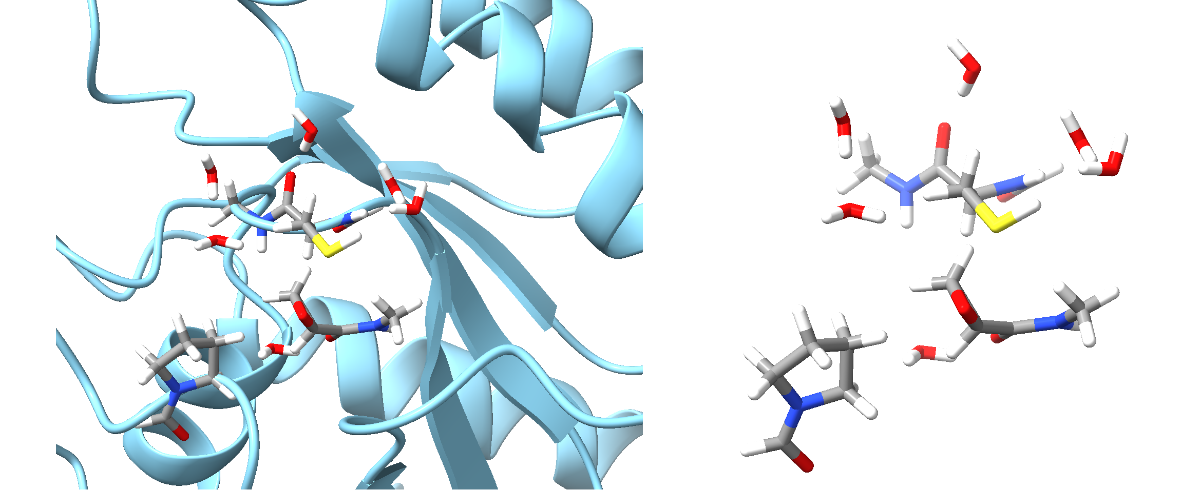
Fig. 6.2 QM region for QMCoreAtoms 183 and 2745. Left is the QM region in ball-and-stick style as part of the full system in cartoon style, right is the QM region with link atoms.
In the above example, involving a covalent ligand bound within a protein active site, we first define the fragments using
the fragmentator, specifying protein-specific groups and functional groups for
ligands and cofactors. We then construct the QM and active regions around the two critical atoms directly involved in
the covalent binding process: atom 183 from the Cys reside, and atom 2745 from the covalently binding ligand.
Keyword |
Options |
Description |
|---|---|---|
|
|
Defines the core atoms of the QM region. Single indices can be given as |
|
|
Defines the core atoms of the active region. |
|
As defined here |
|
|
|
(Default) Take as QM core the atoms that the user defines plus all atoms of the fragments which they belong to. |
|
Take as QM core only the atoms that the user defines. |
|
|
|
(Default) Take as |
|
Take as |
|
|
|
Distance by how much the QM core is extended to yield |
|
|
Check whether two QM atoms show a QM gap, i.e. which are topologically connected by more than |
|
|
Topological distance between two QM atoms which determines whether the connecting MM atoms are considered as a QM gap. Default |
|
|
Check whether a QM-MM bond is an unpolar single bond. If not, add the MM atom’s fragment to |
|
|
(Default) Take as active core the atoms that the user defines plus all atoms of the fragments which they belong to. |
|
Take as active core only the atoms that the user defines. |
|
|
|
(Default) Take as |
|
Take as |
|
|
|
Distance by how much the active core is extended to yield |
|
|
Check whether two active atoms show a gap, i.e. they are topologically connected by more than |
|
|
Check whether an active-nonactive bond is an unpolar single bond. If not, add the non-active atom’s fragment to |
Note
Automated setup can be combined with explicit definition of QM or active atoms via QMAtoms and ActiveAtoms.
6.1.3.3. Definition of QM and Active Region via pdb file
The QM and active region can be defined in the pdb file as shown in the following example:
%qmmm
 Use_QM_InfoFromPDB true     # get the QMAtoms and ActiveAtoms definition from
 Use_Active_InfoFromPDB true # the pdb file. The default for both is false.
                             # If InfoFromPDB is set to true, the QMAtoms or
                             # ActiveAtoms input is ignored
end
*pdbfile 0 1 ubq.pdb
If Use_QM_InfoFromPDB or Use_Active_InfoFromPDB is set to true, a pdb file should be used for
the structural input. QM atoms are defined via 1 in the occupancy
column, MM atoms via 0. Active atoms are defined via 1 in the B-factor
column, non-active atoms via 0.
ubq.pdb:
...
ATOM    327  N   ASP A  21      29.599  18.599   9.828  0.00  0.00      P1   N
ATOM    328  HN  ASP A  21      29.168  19.310   9.279  0.00  0.00      P1   H
ATOM    329  CA  ASP A  21      30.796  19.083  10.566  0.00  1.00      P1   C
ATOM    330  HA  ASP A  21      31.577  18.340  10.448  0.00  1.00      P1   H
ATOM    331  CB  ASP A  21      31.155  20.515  10.048  2.00  1.00      P1   C
ATOM    332  HB1 ASP A  21      30.220  21.082   9.865  2.00  1.00      P1   H
ATOM    333  HB2 ASP A  21      31.754  21.064  10.801  2.00  1.00      P1   H
ATOM    334  CG  ASP A  21      31.923  20.436   8.755  1.00  1.00      P1   C
ATOM    335  OD1 ASP A  21      32.493  19.374   8.456  1.00  1.00      P1   O
ATOM    336  OD2 ASP A  21      31.838  21.402   7.968  1.00  1.00      P1   O
ATOM    337  C   ASP A  21      30.491  19.162  12.040  0.00  0.00      P1   C
ATOM    338  O   ASP A  21      29.367  19.523  12.441  0.00  0.00      P1   O
...
Note
Contrary to the hybrid36 standard of PDB files, ORCA writes non-standard pdb files as:
atoms 1-99,999 in decimal numbers
atoms 100,000 and beyond in hexadecimal numbers, with atom 100,000 corresponding to index 186a0.
This ensures a unique mapping of indices. If you want to select an atom with an index in hexadecimal space (index larger than 100,000), convert the hexadecimal number into decimals when choosing this index in the ORCA input file. Note also, that in the pdb file, counting starts from 1, while in ORCA counting starts from zero.
6.1.4. Active Atoms in Combination with Optimization, Frequency Calculation, MD
The systems of multiscale calculations can become quite large with tens and hundreds of thousands of atoms. In multiscale calculations the region of interest is often only a particular part of the system, and it is common practice to restrict the optimization to a small part of the system, which we call the active region = active part of the system. For info on how to define the active region see QM and Active Region Definition. Usually this active part consists of hundreds of atoms, and is defined as the QM region plus a layer around the QM region. The same definition holds for frequency calculations, in particular since after optimization non-active atoms are not at stationary points, and a frequency calculation would lead to artifacts in such a scenario. MD calculations on systems with hundreds of thousands of atoms are not problematic, but there are applications where a separation in active and non-active parts can be important (e.g. a solute in a solvent droplet, with the outer shell of the solvent frozen).
Note
If no active atoms are defined, the entire system is treated as active.
Note
The active region definitions also apply to MM calculations, but
have to be provided via the %qmmm block.
6.1.4.1. Optimization in redundant internal coordinates
In ORCA’s QM/MM geometry optimization only the positions of the active atoms are optimized. The forces on these active atoms are nevertheless influenced by the interactions with the non-active surrounding atoms. In order to get a smooth optimization convergence for quasi-Newton optimization algorithms in internal coordinates, it is necessary that the Hessian values between the active atoms and the directly surrounding non-active atoms are available. For that reason the active atoms are extended by a shell of surrounding non-active atoms which are also included in the geometry optimization, but whose positions are constrained, see Fig. 6.3. This shell of atoms can be automatically chosen by ORCA. There are three options available:
Keyword |
Options |
Description |
|---|---|---|
|
|
(Default) The parameter |
|
All (non-active) atoms that are covalently bonded to active atoms are included. |
|
|
No non-active atoms are included. |
The user can also provide the atoms for the extension shell manually. This will be discussed in section Frequency Calculation.

Fig. 6.3 Active and non-active atoms. Additionally shown is the extension shell, which consists of non-active atoms close in distance to the active atoms. The extension shell is used for optimization in internal coordinates and PHVA.
The set of active atoms is called the ‘activeRegion’, and the set of active atoms plus the surrounding non-active atoms is called ‘activeRegionExt’. During geometry optimization the following trajectories are stored (which can be switched off):
Filename |
Description |
|
Entire QM/MM system |
|
Only QM region |
|
Only active atoms |
|
Active atoms plus extension |
The following files are stored containing the optimized structures - if requested:
Filename |
Description |
|
Optimized QM/MM system in pdb file format |
|
Optimized QM/MM system |
|
Only QM region |
|
Only active atoms |
|
Active atoms plus extension |
6.1.4.2. Optimization with the Cartesian L-BFGS Minimizer
For very large active regions the quasi-Newton optimization in internal
coordinates can become costly. It can be advantageous to use the
L-Opt or L-OptH feature, see section
Geometry Optimizations using the L-BFGS Optimizer.
In the context of multiscale simulations it can also be useful to treat
parts of the system or full molecules of the system as rigid.
E.g. you can optimize the hydrogen positions of the protein and water
molecules, and at the same time relax non-standard molecules, for
which no exact bonded parameters are available, as rigid bodies.
For available options in that context see Optimization Assuming a Rigid Body.
An example is shown here:
!QMMM L-OptH
%qmmm
 QMAtoms {22397:22423} end
 ORCAFFFilename "DNA_hexamer.ORCAFF.prms"
end
*pdbfile 0 1 DNA_ligand.pdb

%frag
 Definition
  1 {22307:22396} end # cofactor
  2 {22397:22423} end # ligand
 end
end

%geom
 RigidFrags {1 2} end # treat cofactor and ligand as individual rigid bodies
end
6.1.4.3. Frequency Calculation
If all atoms are active, a regular frequency calculation is carried out
when requesting !NumFreq. If there are also non-active atoms in the
QM/MM system, the Partial Hessian Vibrational Analysis (PHVA) is
automatically selected. Here, the PHVA is carried out for the above defined
activeRegionExt, where the extension shell atoms are automatically used
as ‘frozen’ atoms. Note that the analytic Hessian is not available due
to the missing analytic second derivatives for the MM calculation. Note
that in a new calculation after an optimization it might happen that the
new automatically generated extended active region is different compared
to the previous region before optimization. This means that when using a
previously computed Hessian (e.g. at the end of an optimization or a
NEB-TS run) the Hessian does not fit to the new extended active region.
ORCA tries to solve this problem by fetching the information on the
extended region from the .hess file. If that does not work (e.g. if you
distort the geometry after the Hessian calculation) you should manually
provide the list of atoms of the extended active region. This is done
via the following keyword:
%qmmm
 OptRegion_FixedAtoms {27 1288:1290 4400} end  # manually define the
                                               # activeRegionExt atoms.
end
Note that ORCA did print the necessary information in the output of the calculation in which the Hessian was computed:
Fixed atoms used in optimizer ... 27 1288 1289 1290 4400
6.1.4.4. Nudged Elastic Band Calculations
NEB calculations (section Nudged Elastic Band Method) can be carried out in combination with the multiscale features in order to e.g. study enzyme catalysis. When automatically building the extension shell at the start of a Multiscale-NEB calculation, not only the coordinates of the main input structure (‘reactant’), but also the atomic coordinates of the ‘product’ and, if available, of the ‘transition state guess’ are used to determine the union of the extension shell of the active region. For large systems it is advised to use the active region feature for the NEB calculation.
Note
The atomic positions of the non-active atoms of reactant and product and, if available, transition state guess, should be identical.
6.1.4.5. Molecular Dynamics
If there are active and non-active atoms in the multiscale system, only the active atoms are allowed to propagate in the MD run. If all atoms are active, all atoms are propagated. For more information on the output and trajectory options, see section Regions.
6.1.5. Boundary Region
This section is important for the QM/MM, QM/QM2 and QM/QM2/MM methods. For the latter method two boundary regions are present (between QM and QM2 as well as between QM2 and MM region), and both can go through covalent bonds. In the following we will only discuss the concept for the boundary between QM and MM, but the same holds true for the other two boundaries.
6.1.5.1. Link Atoms
ORCA automatically generates link atoms based on the information of the
QM region and on the topology of the system (based on the ORCAFF.prms
file). ORCA places link atoms on the bond between QM and MM atoms.
Important
When defining the QM, QM2 and MM regions, make sure that you only cut through single bonds (not aromatic, double, triple bonds, etc.).
The distance between QM atom and link atom is determined via a bond length scaling factor (in relation to the QM-MM bond length) that is computed as the ratio of the equilibrium bond length between QM and hydrogen atom (\(d_{QM-H}\)) and the equilibrium bond length between QM and MM atom (\(d_{QM-MM}\)).
For the equilibrium bond lengths to hydrogen, ORCA uses tabulated
standard values for the most common atoms involved in boundary regions
(C, N, O), which can be modified via keywords as defined further
below. ORCA stores these values on-the-fly in a simple file
(basename.H_DIST.prms). If necessary, the user can modify these values
atom-specific or add others to the file and provide this file as input
to ORCA (see also
paragraph Get standard hydrogen bond lengths: getHDist). For QM/QM2 and QM/QM2/MM
methods the equilibrium bond lengths to hydrogen are explicitly
calculated.
%qmmm
# standard equilibrium bond lengths with hydrogen can be modified
 Dist_C_HLA 1.09        # d0_C-H
 Dist_O_HLA 0.98        # d0_O-H
 Dist_N_HLA 0.99        # d0_N-H
# file can be provided which provides the used d0_X-H values specific to all atoms
 H_Dist_FileName "QM_H_dist.txt"
end
6.1.5.2. Bonded Interactions at the QM-MM Boundary
The MM bonded interactions within the QM region are neglected in the additive coupling scheme. However, at the boundary, it is advisable to use some specific bonded interactions which include QM atoms. By default ORCA neglects only those bonded interactions at the boundary, where only one MM atom is involved, i.e. all bonds of the type QM1-MM1, bends of the type QM2-QM1-MM1, and torsions of the type QM3-QM2-QM1-MM1. Other QM-MM mixed bonded interactions (with more than two MM atoms involved) are included. The user is allowed to include the described interactions, which is controlled via the following keywords:
%qmmm
 DeleteLADoubleCounting true     # Neglect bends (QM2-QM1-MM1) and torsions
                                 # (QM3-QM2-QM1-MM1). Default true.
 DeleteLABondDoubleCounting true # Neglect bonds (QM1-MM1)
end
6.1.5.3. Charge Alteration
If QM and MM atoms are connected via a bond (defined in the topology
file), the charge of the close-by MM atom (and its neighboring atoms)
has to be modified in order to prevent overpolarization of the electron
density of LA and QM region. This charge alteration is automatically
taken care of by ORCA in %qmmm block. ORCA provides the most popular schemes that can
be used to prevent overpolarization.
Keyword |
Options |
Description |
|---|---|---|
|
|
(Default) Charge Shift – Shift the charge of the MM atom away to the MM2 atoms so that the overall charge is conserved. |
|
Redistributed Charge and Dipole – Shift the charge of the MM atom so that the overall charge and dipole are conserved. |
|
|
Keep charges as they are. This MM atom will probably lead to overpolarization. |
|
|
Delete the charge on the MM1 atom (no overall charge conservation). |
|
|
Delete the charges on the MM1 atom and on its first (MM2) neighbors (no overall charge conservation). |
|
|
Delete the charges on the MM1 atom and on its first (MM2) and second (MM3) neighbors (no overall charge conservation). |
|
|
|
For |
|
|
For |
6.1.6. Embedding Types
There are two embedding schemes available for treating the electrostatic interaction between high level and low level region. In the electrostatic embedding scheme the electrostatic interaction between QM and MM system is computed at the QM level. Thus, the charge distribution of the MM atoms (or other low level methods) can polarize the electron density of the QM region. The following embeding schemes are available:
Keyword |
Options |
Description |
|---|---|---|
|
|
(Default) The electrostatic interaction between the QM and MM system is computed at the QM level. |
|
The electrostatic interaction between the QM and MM system is computed at the MM level. |
Important
In QMMM the LJ interaction between QM and MM system is always computed at the MM level.
In the scheme of electrostatic embedding, the evaluation of the electrostatic potential generated by the MM part can be accelerated by using the FMM algorithm (described in reference [799]). This will speed up the building of the Fock Matrix. The default recommended setup can be called using the FMM-QMMM keyword directly in the keywords line. However, more details about the algorithm parameters and all input options can be found in (see also paragraph Fast Multipole Method)
! FMM-QMMM
It is recommended to use that option whenever the MM part is composed of more than 10,000 atoms (or point charges for ECM methods).
6.1.7. Additional Keywords
Here we list additional keywords and options that are accessible from
within the %qmmm block and that are relevant to QM/MM calculations.
Some of these keywords can also be accessed via the %mm block, see
section Available Keywords for the MM module.
!QMMM
%qmmm

# The extended active region, activeRegionExt, contains the atoms surrounding the
# active atoms.
 ExtendActiveRegion distance  # rule to choose the atoms belonging
                              # to activeRegionExt.
                              # no - do not use activeRegionExt atoms
                              # cov_bonds - add only atoms bonded covalently to
                              # active atoms
                              # distance (default) - use a distance criterion (VDW
                              # distance plus Dist_AtomsAroundOpt)
 Dist_AtomsAroundOpt 0.0      # in Angstrom (Default 0). Meaning only freeze atoms
                              # which touch the active atoms by their VDW spheres.
                              # only needed for ExtendActiveRegion distance
 OptRegion_FixedAtoms {27 1288:1290 4400} end  # manually define the
                                               # activeRegionExt atoms.
                                               # Default: empty list.

# Printing options. All are true by default.
 PrintLevel 1               # Can be 0 to 4, 0=nothing, 1=normal, ...
 PrintOptRegion true        # Additionally print xyz and trj for opt region
 PrintOptRegionExt false    # Additionally print xyz and trj for extended
                            # opt region
 PrintQMRegion true         # Additionally print xyz and trj for QM region
 PrintFullTRJ true          # Print trajectory of full system. Default true.
 PrintPDB true              # Additionally print pdb file for entire system, is
                            # updated every iteration for optimization

# Computing MM nonbonded interactions within non-active region.
 Do_NB_For_Fixed_Fixed true # Compute MM-MM nonbonded interaction also for
                            # non-active atom pairs. Default true.
# Treats all active water molecules that are treated on MM level as rigid bodies
#  in optimization and MD simulation, see section "Rigid Water".
 Rigid_MM_Water false       #  Default false.

end

*pdbfile 0 1 ubq.pdb  # structure input via pdb file, but also possible via
                      # xyz file
Keyword |
Options |
Description |
|---|---|---|
|
|
Filename of the ORCA Force Field prms file. |
|
|
Compute MM-MM nonbonded interaction also within the non-active region (i.e., for non-active atom pairs). Default |
|
|
Optimization and MD of active MM waters. Default |
|
|
Use a distance criterion (VDW distance plus |
|
Add only atoms covalently bonded to active atoms. |
|
|
Do not add any atoms to the extended active region. |
|
|
|
Distance (in Å) to add to VDW radius for |
|
|
List of atoms to define the extended active region. Default: empty list. |
|
|
Additionally print |
|
|
Additionally print |
|
|
Additionally print |