5.39. Static Ground State DFT (SGS-DFT)
5.39.1. Suitability of SGS-DFT for X-ray Spectroscopy
SGS-DFT reduces the complexity of many-electron systems to a one-electron framework by leveraging the Kohn-Sham equations, focusing on electron density that is used to compute ground-state orbitals. In this concept, excited state problems can be constructed on the basis of orbital energy differences, in strict difference to excited state methodologies (e.g., TD-DFT, ROCIS, RASCI/CASCI/NEVPT2, MRCI/MREOM-CC). This simplicity makes it computationally efficient while still providing reliable results in a number of X-ray spectroscopy experiments, such as X-ray Absorption Spectroscopy (XAS), X-ray Emission Spectroscopy (XES), and Resonant Inelastic X-ray Scattering (RIXS).
SGS-DFT has found significant applications in Valence-to-Core X-ray Emission Spectroscopy (VtC-XES), which probes valence orbitals via core-hole transitions, offering insights into ligand-metal interactions. It complements other one-electron methods like TD-DFT for XAS, as well as wavefunction-based approaches (ROCIS, RASCI/CASCI/NEVPT2, MRCI/MREOM-CC) and Ligand Field-based CI methods, balancing accuracy and computational cost. A collective review about all these methodologies their advantages and their limitationsisin computing X-ray spectroscopy spectra is provided in reference [454].
5.39.2. Summary of Cross Section Equations
In this section we sumarize the general, non-relativistic and releativistic expressions for cross sections in X-ray spectroscopy, including XAS, XES, and RIXS.
Indices and Notations
\(\rho, \rho'\): Cartesian components of the dipole moment, summing over \(x, y, z\), i.e., \(\rho, \rho' \in {x, y, z}\).
\(I\): Initial state (ground state in general expressions).
\(F\): Final state in general cross-section and XAS expressions, with summation over \(F\) including all possible final states.
\(V, V'\): Intermediate states in RIXS expressions, with energies \(\epsilon_V, \epsilon_{V'}\).
\(i_\sigma, j_\sigma\): Occupied 1-electron orbitals in non-relativistic treatment, where \(\sigma \in {\alpha, \beta}\) denotes spin.
\(a_\sigma\): Unoccupied 1-electron orbitals in non-relativistic treatment, with \(\sigma \in {\alpha, \beta}\).
\(\nu_\sigma, \nu'_\sigma\): Intermediate states in non-relativistic RIXS expressions, with \(\sigma \in {\alpha, \beta}\).
\(\omega_{ex}\): Excitation energy (incident radiation frequency).
\(\omega_{em}\): Emission energy (scattered radiation frequency in XES).
\(\omega_{sc}\): Scattering energy (used in RIXS for scattered radiation frequency).
\(\Delta \omega\): Energy transfer in RIXS, typically \(\Delta \omega = \omega_{ex} - \omega_{sc}\).
\(\omega_{FI}\): Transition energy between initial state \(I\) and final state \(F\).
\(\omega_{VI}\): Transition energy between initial state \(I\) and intermediate state \(V\).
\(\omega_{a_\sigma i_\sigma}\): Transition energy between unoccupied orbital \(a_\sigma\) and occupied orbital \(i_\sigma\), defined as \(\epsilon_{a_\sigma} - \epsilon_{i_\sigma}\).
\(\omega_{j_\sigma i_\sigma}\): Transition energy between occupied orbitals \(j_\sigma\) and \(i_\sigma\), defined as \(\epsilon_{j_\sigma} - \epsilon_{i_\sigma}\).
\(\epsilon_{a_\sigma}, \epsilon_{i_\sigma}, \epsilon_{\nu_\sigma}, \epsilon_{\nu'\sigma}\): Orbital energies for unoccupied orbital \(a\sigma\), occupied orbital \(i_\sigma\), and intermediate states \(\nu_\sigma, \nu'_\sigma\).
\(\Gamma, \Gamma_{\nu_\sigma}, \Gamma_{\nu'_\sigma}\): Linewidth parameters for lifetime broadening.
\(\Gamma_F\): Linewidth parameter for final state \(F\).
\(c\): Speed of light (\(\sim 137\) in atomic units).
\(m\): Electric dipole transition operator, defined as \(m = \sum_i \mathbf{r}_i + \sum_A \mathbf{Z}_A \mathbf{R}_A\), where \(\mathbf{r}_i\) are electron coordinates and \(\mathbf{Z}_A \mathbf{R}_A\) are nuclear contributions.
General Expressions
XAS Cross Section
The XAS cross section, describing absorption from initial state \(I\) to final state \(F\), is:
or equivalently:
XES Cross Section
The XES cross section, describing emission from an intermediate state to a final state \(F\), is:
RIXS Cross Section
The inelastic scattering cross section for RIXS is:
Polarizability Tensor
The polarizability tensor from the Kramers-Heisenberg-Dirac expression is:
5.39.3. Orbitals, States, and Energies
The present treatment is based on a single one-electron approach. The orbitals come from a density functional theory (DFT) calculation and satisfy the Kohn-Sham equations
where \(F^{\text{KS}}\) is the Kohn-Sham operator, \(| \rho_{\mathbf{k}} \rangle\) is a spin-orbital with spin \(\sigma_{\mathbf{k}} = 0, \beta\) and \(\varepsilon_{\mathbf{k}}\) is the orbital energy. The Kohn-Sham operator is:
where \(h\) is the one-electron Hamiltonian (kinetic energy plus electron-nuclear potential together with possibly present other external potentials), the second term presents the Coulomb repulsion where
is the electron density and the exchange correlation potential is:
The quantity \(E_{\text{xc}} [\rho]\) is the exchange-correlation functional. Associated with the Kohn-Sham procedure is the Kohn-Sham determinant:
In general, occupied orbitals of the electronic ground state are labeled with \(i,j,k,\ldots\) and unoccupied ones with \(a,b,c,\ldots\). In the one-electron approach, the initial, intermediate, and final states are constructed as:
In the specific application at hand, orbital \(i\) is a core-orbital, e.g., the metal 1s derived orbital of a given absorber atom, \(a\) is an arbitrary unoccupied orbital (but most importantly an empty metal d-based orbital) and \(j\) is another core-level orbital of the same atom.
Rather than trying to obtain accurate total energies for all of these states, the simple approximations are adopted:
This is of course fairly simplistic. In terms of time-dependent DFT, it can be shown that the orbital energy difference is a well-defined approximation to the state energy difference if no Hartree-Fock exchange is present in the DFT potential. For a semi-quantitative discussion it should be good enough since the substantial errors of the presently used DFT potentials prevent the calculations from predicting accurate transition energies anyways.
5.39.4. Non-Relativistic Treatment in 1-Electron Orbital Basis
In the non-relativistic treatment, states are expressed using 1-electron orbitals. The initial state is a Slater determinant of occupied orbitals \(i_\sigma\), and the final state involves excitations to unoccupied orbitals \(a_\sigma\), with \(\sigma \in {\alpha, \beta}\) denoting the spin.
Non-Relativistic XAS
The non-relativistic XAS cross section is:
or equivalently:
Non-Relativistic XES
The non-relativistic XES cross section is:
Non-Relativistic Polarizability Tensor
The non-relativistic polarizability tensor is:
Alternatively, if \(\omega_{\text{ex}}\) is tuned to resonance with an intermediate state, the dominant term is:
Along the \(\omega_{\text{sc}}\) axis, this is a resonance centered at \(\varepsilon_j^\sigma - \varepsilon_a^\sigma\). This suggests providing a list of \((i_\sigma, j_\sigma)\) with transition energies \(E_{\omega_{\text{ex}}} = \varepsilon_a^\sigma - \varepsilon_i^\sigma\), \(E_{\omega_{\text{sc}}} = \varepsilon_a^\sigma - \varepsilon_j^\sigma\), and values \(\left| \langle a_\sigma | m_\rho | i_\sigma \rangle \right|^2 \left| \langle i_\sigma | m_\lambda | j_\sigma \rangle \right|^2\). Tools like orca_mapspc can read the linewidth and convolute peaks with a lineshape function, such as:
This emphasizes that RIXS effectively measures L or M-edges through excitation at, e.g., the K-edge. Other lineshapes (Lorentzian, Gaussian, Voigt) are possible, as explained in sections (placeholder mapspc).
Non-Relativistic RIXS
Hence the non-relativistic RIXS cross section becomes:
5.39.5. Inclusion of Relativistic Effects
There are two leading types of relativistic effects: scalar relativistic (spin free) relativistic effects and spin-orbit coupling.
Scalar Relativistic Effects
Scalar relativistic effects can be included employing various schemes as described in Relativistic Calculations by modifying the one-electron part of the HamiltonianThe scalar relativistic effects show up as an attractive potential close to the nucleus. Hence \(s\)-, and \(p\)-orbitals are stabilized, \(d\)- and \(f\)-orbitals are destabilized. Concomitant with these effects, the radial functions of \(s\)- and \(p\)-orbitals will contract those of \(d\)-orbitals will expand. Hence, transition dipole moments will also be modified
Spin-Orbit Coupling (SOC)
The spin-orbit coupling is much more problematic since the SOC is a two-electron operator that couples different spin-manifold and pure-spin multiplets. A good approximation is the spin-orbit meanfield (SOMF) treatment The Spin-Orbit Coupling Operator In this case, the SOC shows up as an effective one-electron operator of the form::
\(H_{\text{SOMF}} = \sum_{\mathbf{k}} h^{\text{SOC}} s_{\mathbf{k}}\)
Inclusion of SOC in 1-electron framework
In \textit{ab initio} quantum chemistry one can use the Wigner–Eckart algebra in order to explicitly couple all \(M_s\) substates for states of total spin \(S\). This corresponds roughly to LS coupling in the atomic case. For the SGS-DFT approach that we use here this is not an option and hence we are tied to \(jj\) coupling type treatments. The more rigorous version of this approach are two-component DFT approaches. Here we try a simple version of this more elaborate procedure. It consists of diagonalizing the Kohn–Sham and SOC operators in the basis of the converged non- or scalar relativistic spin-orbitals. Hence, the eigenvalue equation is:
The matrix elements are in more detail:
The matrix elements \(L_{pq}\), are the spatial parts of the SOC operator and have the property that they are antisymmetric \(L_{pq} = -L_{pq}\).
The diagonalization of this complex Hermitian matrix yields SOC corrected orbital energies and `two component’ orbitals that are linear combinations of the spin-free spin-orbitals:
From these orbitals one readily calculates the transition moments:
where the \(V\)’s are the eigenfunctions of the \(\mathbf{F} + \mathbf{h}^{\text{SOC}}\) matrix. With these transition moments and orbital energies all XAS, XES and RIXS is computed as before; one simply has the spin-orbit label \(p\).
5.39.6. Computations of X-ray Spectroscopic Properties
In the following examples we present a variety of X-ray spectroscopic employing the conventional BP86 in conjuctuon with the X2C relativstic hamiltonian and the reseoctive triple-zeta basis set. However in principle any relativistic scheme can be used instead Basis Sets in Relativistic Calculations
We choose to describeexplicitely the X-ray computed spectra of the octagedral \(\mathrm{Fe}^{\mathrm{III}}\) complex \([\mathrm{Fe}^{\mathrm{III}}\mathrm{Cl}_6]^{3-}\).
!BP86 X2C x2c-TZVPall-s x2c/J

%xes
 #-------------------------------
 #    General Definitions
 #-------------------------------
 CoreOrb 0,0
 OrbOp 0,1
 CoreOrbSOC 0,1
 #-------------------------------
 #    Spectroscopic Properties
 #-------------------------------
 DoXAS true
 DoSOC true
 #-------------------------------
 #    Spectra Intensities
 #-------------------------------
 DoDipoleLength true
 DoFullSemiclassical true
end

* xyz -1 6
Fe      -0.008368229      0.000000000      0.012210784
Cl      -1.375773751     -1.142123897     -0.186609497
Cl      -0.530592683      1.387798468      1.019718298
Cl       0.513856225      0.592852206     -1.597007114
Cl       1.359037292     -0.838526778      0.812741448
*
As the core of the SCF-XES or SGS-XES method involves the derivation of all important quantities in orbital and spin-orbital basis for computing the K-edge Fe XAS as well as the resepctive Mainline XES and the corresponding (Valence to Core) VtC-XES spectra one chooses the list of the desired core orbitals here the \(\mathrm{Fe}_{1s}\) with the resepctive Orbital (0 and 1) and SOC Orbital operators (here 0 and 1).
 CoreOrb 0,0
 OrbOp 0,1
 CoreOrbSOC 0,1
And we compute both the:
\(K_{\alpha}\): \(\mathrm{Fe}\ 2p \rightarrow \mathrm{Fe}\ 1s\) (Mainline XES)
\(K_{\beta_{1,3}}\): \(\mathrm{Fe}\ 3p \rightarrow \mathrm{Fe}\ 1s\) (Mainline XES)
\(K_{\beta_{2,5}}\) / \(K_{\beta'}\): \((\mathrm{Cl}\ 2p + \mathrm{Fe}\ 3d) \rightarrow \mathrm{Fe}\ 1s\) (VtC-XES)
besides the K-edge Fe XAS spectra
In the non relativistic section one then obtains the XAS and XES spectra within the ORCA’s One-Photon Spectroscopy framework
--------------------------------------
CALCULATION OF X-RAY EMISSION SPECTRUM
--------------------------------------
Reading and Transforming integrals ... Generating transition densities between Orbitals ... done
Reading integrals                                                ...
Reading the Dipole integrals                                     ... done

Calculating the Full-semiclassical Transition moment on transition block:0  ...
10% done
20% done
30% done
40% done
50% done
60% done
70% done
80% done
90% done
100% done
All done in  (       29.14 sec)
--------------------------------------------------------------------
Using One-Photon Spectroscopy Tool
--------------------------------------------------------------------

----------------------------------------------------------------------------------------------------
              X-RAY   EMISSION SPECTRUM VIA TRANSITION ELECTRIC DIPOLE MOMENTS
----------------------------------------------------------------------------------------------------
     Transition      Energy     Energy  Wavelength fosc(D2)      D2        DX        DY        DZ
                      (eV)      (cm-1)    (nm)                 (au**2)    (au)      (au)      (au)
----------------------------------------------------------------------------------------------------
  1a-a  ->  0a-a   4243.560625 34226628.2     0.3   0.000000000   0.00000   0.00000  -0.00000  -0.00000
  2a-a  ->  0a-a   4243.562891 34226646.5     0.3   0.000000000   0.00000   0.00000   0.00000   0.00000
  3a-a  ->  0a-a   4243.563723 34226653.2     0.3   0.000000000   0.00000  -0.00000   0.00000  -0.00000
  4a-a  ->  0a-a   4243.563845 34226654.2     0.3   0.000000000   0.00000   0.00000   0.00000  -0.00000
  1b-a  ->  0b-a   4243.609379 34227021.5     0.3   0.000000000   0.00000   0.00000  -0.00000  -0.00000
  2b-a  ->  0b-a   4243.611639 34227039.7     0.3   0.000000000   0.00000   0.00000   0.00000   0.00000
  3b-a  ->  0b-a   4243.612467 34227046.4     0.3   0.000000000   0.00000   0.00000  -0.00000   0.00000
  4b-a  ->  0b-a   4243.612590 34227047.4     0.3   0.000000000   0.00000   0.00000   0.00000  -0.00000
  5a-a  ->  0a-a   6174.919612 49804090.7     0.2   0.000000000   0.00000  -0.00000   0.00000   0.00000
  5b-a  ->  0b-a   6176.509051 49816910.3     0.2   0.000000000   0.00000  -0.00000   0.00000   0.00000
  6a-a  ->  0a-a   6296.393596 50783844.5     0.2   0.101316564   0.00066  -0.02354   0.00780  -0.00648
  7a-a  ->  0a-a   6296.393628 50783844.8     0.2   0.101316573   0.00066  -0.00668   0.00037   0.02474
  8a-a  ->  0a-a   6296.393675 50783845.1     0.2   0.101316586   0.00066  -0.00762  -0.02441  -0.00169
  6b-a  ->  0b-a   6297.611741 50793669.5     0.2   0.101563788   0.00066   0.02425  -0.00783   0.00303
  7b-a  ->  0b-a   6297.611770 50793669.7     0.2   0.101563797   0.00066  -0.00317   0.00003   0.02546
  8b-a  ->  0b-a   6297.611810 50793670.1     0.2   0.101563807   0.00066  -0.00777  -0.02443  -0.00094

...

-----------------------------------------------------------------------------
              X-RAY   EMISSION SPECTRUM VIA FULL SEMI-CLASSICAL FORMULATION
-----------------------------------------------------------------------------
     Transition      Energy     Energy  Wavelength   fosc(FFMIO)
                      (eV)      (cm-1)    (nm)
-----------------------------------------------------------------------------
  1a-a  ->  0a-a   4243.560625 34226628.2     0.3     0.00000000000264
  2a-a  ->  0a-a   4243.562891 34226646.5     0.3     0.00000000000270
  3a-a  ->  0a-a   4243.563723 34226653.2     0.3     0.00000000000328
  4a-a  ->  0a-a   4243.563845 34226654.2     0.3     0.00000000000163
  1b-a  ->  0b-a   4243.609379 34227021.5     0.3     0.00000000000264
  2b-a  ->  0b-a   4243.611639 34227039.7     0.3     0.00000000000270
  3b-a  ->  0b-a   4243.612467 34227046.4     0.3     0.00000000000327
  4b-a  ->  0b-a   4243.612590 34227047.4     0.3     0.00000000000163
  5a-a  ->  0a-a   6174.919612 49804090.7     0.2     0.00000000000007
  5b-a  ->  0b-a   6176.509051 49816910.3     0.2     0.00000000000006
  6a-a  ->  0a-a   6296.393596 50783844.5     0.2     0.10239197992333
  7a-a  ->  0a-a   6296.393628 50783844.8     0.2     0.10239199025533
  8a-a  ->  0a-a   6296.393675 50783845.1     0.2     0.10239200379726
  6b-a  ->  0b-a   6297.611741 50793669.5     0.2     0.10265622291301
  7b-a  ->  0b-a   6297.611770 50793669.7     0.2     0.10265623313526
  8b-a  ->  0b-a   6297.611810 50793670.1     0.2     0.10265624471656

----------------------------------------
CALCULATION OF X-RAY ABSORPTION SPECTRUM
----------------------------------------
Reading integrals                                                ...
Reading the Dipole integrals                                     ... done

Calculating the Full-semiclassical Transition moment on transition block:0        ...
10% done
20% done
30% done
40% done
50% done
60% done
70% done
80% done
90% done
100% done
All done in  (      105.64 sec)
--------------------------------------------------------------------
Using One-Photon Spectroscopy Tool
--------------------------------------------------------------------

----------------------------------------------------------------------------------------------------
              X-RAY ABSORPTION SPECTRUM VIA TRANSITION ELECTRIC DIPOLE MOMENTS
----------------------------------------------------------------------------------------------------
     Transition      Energy     Energy  Wavelength fosc(D2)      D2        DX        DY        DZ
                      (eV)      (cm-1)    (nm)                 (au**2)    (au)      (au)      (au)
----------------------------------------------------------------------------------------------------
  0b-a  -> 45b-a   6988.978848 56369921.9     0.2   0.000000000   0.00000   0.00000   0.00000  -0.00000
  0b-a  -> 46b-a   6988.978999 56369923.1     0.2   0.000000000   0.00000   0.00000  -0.00000  -0.00000
  0b-a  -> 47b-a   6990.167972 56379512.8     0.2   0.000111632   0.00000  -0.00045   0.00053   0.00040
  0b-a  -> 48b-a   6990.168059 56379513.5     0.2   0.000111638   0.00000  -0.00048  -0.00060   0.00026
  0b-a  -> 49b-a   6990.168100 56379513.8     0.2   0.000111637   0.00000  -0.00047   0.00010  -0.00065
  0a-a  -> 50a-a   6992.570956 56398894.2     0.2   0.000000000   0.00000   0.00000   0.00000   0.00000
  0b-a  -> 50b-a   6992.689756 56399852.4     0.2   0.000000000   0.00000  -0.00000   0.00000   0.00000
  0a-a  -> 51a-a   6995.905926 56425792.5     0.2   0.000037002   0.00000  -0.00036  -0.00006   0.00029
  0a-a  -> 52a-a   6995.906125 56425794.1     0.2   0.000036975   0.00000   0.00006  -0.00046  -0.00003
  0a-a  -> 53a-a   6995.906494 56425797.1     0.2   0.000037064   0.00000  -0.00029  -0.00002  -0.00036
  0a-a  -> 54a-a   6996.058845 56427025.9     0.2   0.000006536   0.00000   0.00010  -0.00009   0.00014
  0a-a  -> 55a-a   6996.059201 56427028.8     0.2   0.000006569   0.00000   0.00016   0.00010  -0.00005
  0a-a  -> 56a-a   6996.059311 56427029.7     0.2   0.000006619   0.00000  -0.00004   0.00014   0.00013
  0b-a  -> 51b-a   6996.206394 56428216.0     0.2   0.000014342   0.00000   0.00021  -0.00015  -0.00013

-----------------------------------------------------------------------------
              X-RAY ABSORPTION SPECTRUM VIA FULL SEMI-CLASSICAL FORMULATION
-----------------------------------------------------------------------------
     Transition      Energy     Energy  Wavelength   fosc(FFMIO)
                      (eV)      (cm-1)    (nm)
-----------------------------------------------------------------------------
  0b-a  -> 45b-a   6988.978848 56369921.9     0.2     0.00000231997701
  0b-a  -> 46b-a   6988.978999 56369923.1     0.2     0.00000232027335
  0b-a  -> 47b-a   6990.167972 56379512.8     0.2     0.00011661916478
  0b-a  -> 48b-a   6990.168059 56379513.5     0.2     0.00011662652902
  0b-a  -> 49b-a   6990.168100 56379513.8     0.2     0.00011662384321
  0a-a  -> 50a-a   6992.570956 56398894.2     0.2     0.00000000000014
  0b-a  -> 50b-a   6992.689756 56399852.4     0.2     0.00000000000008
  0a-a  -> 51a-a   6995.905926 56425792.5     0.2     0.00004544364720
  0a-a  -> 52a-a   6995.906125 56425794.1     0.2     0.00004540088165
  0a-a  -> 53a-a   6995.906494 56425797.1     0.2     0.00004552596978
  0a-a  -> 54a-a   6996.058845 56427025.9     0.2     0.00001087977536
  0a-a  -> 55a-a   6996.059201 56427028.8     0.2     0.00001092658019
  0a-a  -> 56a-a   6996.059311 56427029.7     0.2     0.00001099716202
  0b-a  -> 51b-a   6996.206394 56428216.0     0.2     0.00001669184884
The program the proceeds to generate the SOC corrected orbitals
-----------------------------------------
XES/XAS SPECTRUM WITH SPIN ORBIT COUPLING
-----------------------------------------

Reading the SOC integrals             ... done
Forming the SOC Hamiltonian           ... done
Diagonalizing the SOC Hamiltonian     ... done
-------------------------------
SOC CORRECTED OCCUPIED ORBITALS
-------------------------------
 E[   0] = -6987.772 eV: ( -0.512 +  -0.859 *i)|   0a>
 E[   1] = -6987.756 eV: (  0.002 +  -1.000 *i)|   0b>
 E[   2] = -2744.212 eV: (  0.383 +  -0.924 *i)|   1a>
 E[   3] = -2744.209 eV: ( -0.772 +  -0.636 *i)|   2a>
 E[   4] = -2744.208 eV: ( -0.952 +   0.307 *i)|   3a>
 E[   5] = -2744.208 eV: ( -0.923 +   0.384 *i)|   4a>
 E[   6] = -2744.147 eV: ( -0.001 +  -1.000 *i)|   1b>
 E[   7] = -2744.144 eV: (  0.001 +  -1.000 *i)|   2b>
 E[   8] = -2744.144 eV: (  0.244 +   0.970 *i)|   3b>
 E[   9] = -2744.143 eV: (  0.025 +  -1.000 *i)|   4b>
 E[  10] =  -812.853 eV: (  0.512 +  -0.859 *i)|   5a>
 E[  11] =  -811.247 eV: (  0.163 +   0.987 *i)|   5b>
 E[  12] =  -698.833 eV: (  0.548 +  -0.181 *i)|   6a> (  0.155 +  -0.009 *i)|   7a> (  0.177 +   0.568 *i)|   8a> ( -0.534 +  -0.000 *i)|   7b>
 E[  13] =  -698.431 eV: (  0.072 +  -0.139 *i)|   6a> ( -0.275 +   0.529 *i)|   7a> (  0.393 +  -0.388 *i)|   6b> (  0.392 +   0.394 *i)|   8b>
 E[  14] =  -687.512 eV: ( -0.671 +   0.134 *i)|   6a> ( -0.165 +   0.082 *i)|   7a> (  0.150 +   0.689 *i)|   8a>
 E[  15] =  -687.067 eV: ( -0.092 +   0.176 *i)|   6a> (  0.350 +  -0.673 *i)|   7a> (  0.309 +  -0.305 *i)|   6b> (  0.308 +   0.310 *i)|   8b>
 E[  16] =  -686.654 eV: ( -0.349 +   0.116 *i)|   6a> ( -0.113 +  -0.362 *i)|   8a> ( -0.837 +  -0.000 *i)|   7b>
 E[  17] =  -686.266 eV: (  0.500 +   0.493 *i)|   6b> (  0.499 +  -0.501 *i)|   8b>
in following all spectra are recomputed in the OPS framework in the presence of SOC
Generating transition densities between SOC_Corrected_Orbitals         ... done
------------------------------------------------------
CALCULATION OF SOC CORRECTED X-RAY EMISSION SPECTRUM
------------------------------------------------------
Reading integrals                                                ...
Reading the Dipole integrals                                     ... done

Calculating the Full-semiclassical Transition moment on transition block:0        ...
10% done
20% done
30% done
40% done
50% done
60% done
70% done
80% done
90% done
100% done
All done in  (       58.75 sec)
--------------------------------------------------------------------
Using One-Photon Spectroscopy Tool
--------------------------------------------------------------------

--------------------------------------------------------------------------------------------------------
   SPIN-ORBIT X-RAY   EMISSION SPECTRUM VIA TRANSITION ELECTRIC DIPOLE MOMENTS
--------------------------------------------------------------------------------------------------------
      Transition         Energy     Energy  Wavelength fosc(D2)      D2       |DX|      |DY|      |DZ|
                          (eV)      (cm-1)    (nm)                 (au**2)    (au)      (au)      (au)
--------------------------------------------------------------------------------------------------------
     2-a  ->  0-a      4243.560625 34226628.2     0.3   0.000000000   0.00000   0.00000   0.00000   0.00000
     2-a  ->  1-a      4243.544569 34226498.7     0.3   0.000000000   0.00000   0.00000   0.00000   0.00000
     3-a  ->  0-a      4243.562891 34226646.5     0.3   0.000000000   0.00000   0.00000   0.00000   0.00000
     3-a  ->  1-a      4243.546835 34226517.0     0.3   0.000000000   0.00000   0.00000   0.00000   0.00000
     4-a  ->  0-a      4243.563723 34226653.2     0.3   0.000000000   0.00000   0.00000   0.00000   0.00000
     4-a  ->  1-a      4243.547667 34226523.7     0.3   0.000000000   0.00000   0.00000   0.00000   0.00000
     5-a  ->  0-a      4243.563845 34226654.2     0.3   0.000000000   0.00000   0.00000   0.00000   0.00000
     5-a  ->  1-a      4243.547790 34226524.7     0.3   0.000000000   0.00000   0.00000   0.00000   0.00000
     6-a  ->  0-a      4243.625435 34227151.0     0.3   0.000000000   0.00000   0.00000   0.00000   0.00000
     6-a  ->  1-a      4243.609379 34227021.5     0.3   0.000000000   0.00000   0.00000   0.00000   0.00000
     7-a  ->  0-a      4243.627694 34227169.2     0.3   0.000000000   0.00000   0.00000   0.00000   0.00000
     7-a  ->  1-a      4243.611639 34227039.7     0.3   0.000000000   0.00000   0.00000   0.00000   0.00000
     8-a  ->  0-a      4243.628523 34227175.9     0.3   0.000000000   0.00000   0.00000   0.00000   0.00000
     8-a  ->  1-a      4243.612467 34227046.4     0.3   0.000000000   0.00000   0.00000   0.00000   0.00000
     9-a  ->  0-a      4243.628646 34227176.9     0.3   0.000000000   0.00000   0.00000   0.00000   0.00000
     9-a  ->  1-a      4243.612590 34227047.4     0.3   0.000000000   0.00000   0.00000   0.00000   0.00000
    10-a  ->  0-a      6174.919612 49804090.7     0.2   0.000000000   0.00000   0.00000   0.00000   0.00000
    10-a  ->  1-a      6174.903556 49803961.2     0.2   0.000000000   0.00000   0.00000   0.00000   0.00000
    11-a  ->  0-a      6176.525107 49817039.8     0.2   0.000000000   0.00000   0.00000   0.00000   0.00000
    11-a  ->  1-a      6176.509051 49816910.3     0.2   0.000000000   0.00000   0.00000   0.00000   0.00000
    12-a  ->  0-a      6288.939050 50723719.5     0.2   0.072768392   0.00047   0.01537   0.01537   0.00000
    12-a  ->  1-a      6288.922994 50723590.0     0.2   0.029738152   0.00019   0.00000   0.00000   0.01389
    13-a  ->  0-a      6289.340683 50726958.9     0.2   0.039112694   0.00025   0.00000   0.00000   0.01593
    13-a  ->  1-a      6289.324627 50726829.4     0.2   0.063473047   0.00041   0.01435   0.01435   0.00000
    14-a  ->  0-a      6300.260175 50815030.6     0.2   0.100751569   0.00065   0.01807   0.01807   0.00000

...

and so on for the rest of the spectra tables
All Spectra are generated using orca_mapspc with [Options] for XAS, XES, XASFFMIO and XESSFFMIO, including electric dipole (ED), with full field matter interaction operator (FFMIO) with and without SOC:
orca_mapspc FileName.out [Options] -x06000 -x18000 -w2.0 -n10000
The computed XAS spectra in the electric dipole approximation EDA, and employing the FFMIO semicalssical operator with and wthout SOC are shown in Figure Fig. 5.73.
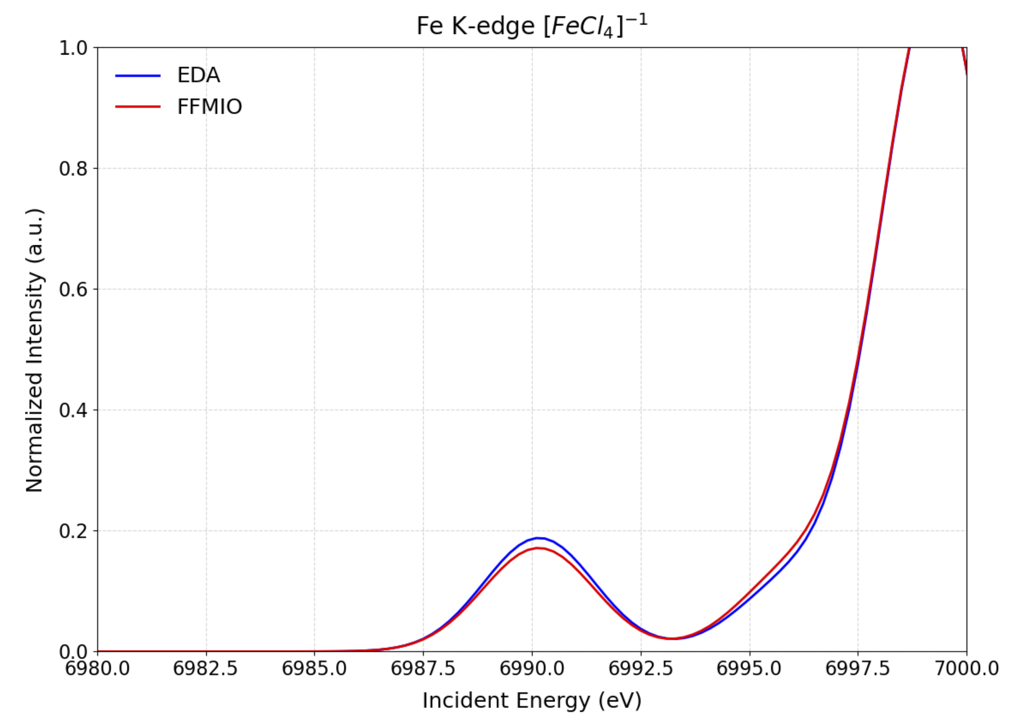
Fig. 5.73 Comparison of the calculated SGS-DFT Fe K-edge XAS spectra of \([FeCl_4]^{1-}\). within the EDA (blue) and FFMIO (red) approximations.
In following the computed \(K_{\alpha}\): Mainline XES spectra employing the FFMIO semicalssical operator with and wthout SOC are shown in Figure Fig. 5.74. In the case of SOC one observes explicitely the SOC splitting owning to the 2p core-hole in the 2p \(\rightarrow \mathrm{Fe}\ 1s\) (Mainline XES) electron decay process.
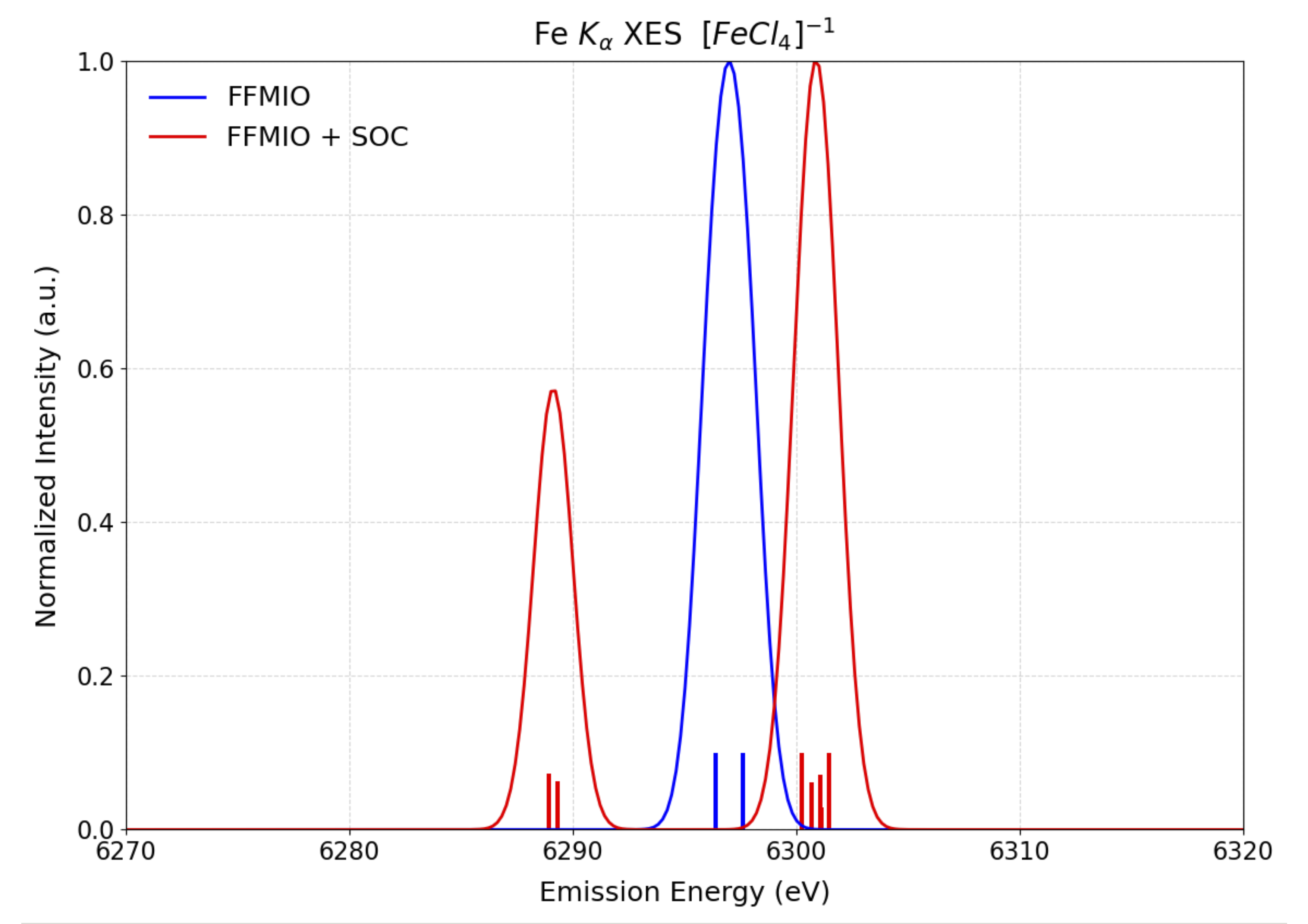
Fig. 5.74 Comparison of the calculated SGS-DFT \(K_{\alpha}\): Mainline XES spectra of \([FeCl_4]^{1-}\). employing the FFMIO semicalssical operator with SOC (red) and without SOC (blue) corrections.
in this state to orbital approach where in principle every orbital excitation constitute a state withing the SGS-DFT framework, in the same
calculation setup, one also obtains in addition all accesible electron decay processes. This means that in addition to the
\(K_{\beta_{1,3}}\): \(\mathrm{Fe}\ 3p \rightarrow \mathrm{Fe}\ 1s\) (Mainline XES) as well as the
\(K_{\beta_{2,5}}\) / \(K_{\beta'}\): \((\mathrm{Cl}\ 2p + \mathrm{Fe}\ 3d) \rightarrow \mathrm{Fe}\ 1s\) (VtC-XES)
maybe accessed as is shown in Figure Fig. 5.75.
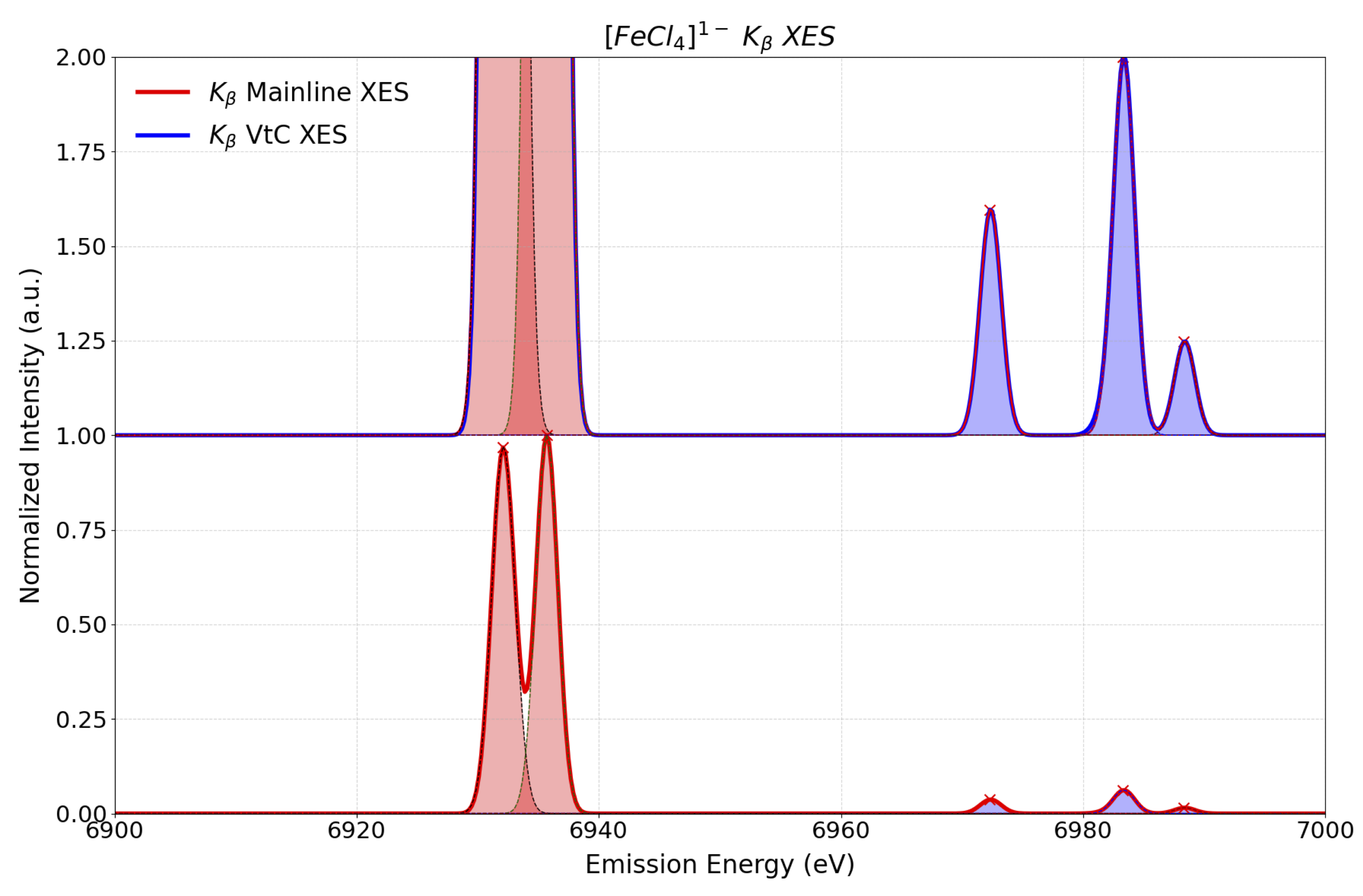
Fig. 5.75 Calculated SGS-DFT \(K_{\beta}\): Mainline XES (red) and VtC XES (blue) spectra of \([FeCl_4]^{1-}\). employing the FFMIO semicalssical operator with SOC corrections
In the same framework one can also compute Simple RIXS spectra in the Direct RIXS fashion… To become available in the next minor release. For more information about the RIXS spectra theory and generation please have a look in section: Resonant Inelastic Scattering Spectroscopy
The entire keyword setup in the %xes block of SCF-XES or SSS-DFT method is given below
%xes
 #-------------------------------
 #    Core Orbital Definitions
 #-------------------------------
 CoreOrb 0,0 # list of core orbitals (alpha,-beta)
 OrbOp 0,1 # operators for core-orbitals (0=alpha,1=beta)
 CoreOrbSOC 0,1 # core orbitals for SOC calculations
 #-------------------------------
 #    RIXS Orbital Definitions
 #-------------------------------
 RIXSOrb    6,7,8,6,7,8       # RIXS final orbitals
 RIXSOrbOp  0,0,0,1,1,1       # operators for these orbitals
 RIXSOrbSOC 12,13,14,15,16,17 # same for SOC
 #-------------------------------
 #    Virtual Orbital Definitions
 #-------------------------------
 MaxNVirt 200 #max number of virtual Orbitals
 #-------------------------------
 #    Spectroscopic Properties
 #-------------------------------
 DoXAS true # Do calculate XAS spectra in addition to XES
 DoSOC true # Do calculate SOC corrected  spectra
 DoRIXS true # Do calculate RIXS  spectra
 #-------------------------------
 #    Spectra Intensities
 #-------------------------------
 DoDipoleLength true # Calculate Spectra in Electric Dipole EDA (Length/Velocity)
 DoFullSemiclassical true # Calculate Spectra in Semiclassical FFMIO framework
end
Note
It is in general not recomended to compute X-ray spectra with complex multiplet structure via the SGS-DFT approach. This involves e.g. metal L/M-edge XAS spectra, \(K_{\alpha}\): \(\mathrm{Fe}\ 2p \rightarrow \mathrm{Fe}\ 1s\) and \(K_{\beta_{1,3}}\): \(\mathrm{Fe}\ 3p \rightarrow \mathrm{Fe}\ 1s\) (Mainline XES) as well as RIXS spectra. The computation of such spectroscopic problem is preferably tackled on the basis of wavefunction methodologies:
ROCIS and CASCI/RASCI (in combination with NEVPT2) or multirefernce approaches (e.g. MREOM-CC) and MCRPA are able to tackle a variety of such complex spectroscopes, see discussions in Transition Metal L-Edges with ROCIS or DFT/ROCIS, Resonant Inelastic Scattering Spectroscopy, Core Excited Spectra: CAS-CI/RAS-CI XES, Excited States via MCRPA
In a similar framework TD-DFT has been proven instrumental in computing metal and ligand K-edge spectra, see discussions in Excited States via RPA, CIS, TD-DFT and SF-TDA.
Core level spectroscopy spectra (presently Metal/Ligand K-edge XAS) can also be computed with couple-cluster (EOM-CC, STEOM-CC) methods see discussions in Core-Level Spectroscopy with Coupled Cluster Methods