3.4. Density Functional Theory (DFT)

Due to its good cost-accuracy ratio, Kohn-Sham density functional theory (DFT) has become the workhorse of quantum chemistry. Over the last few decades, a whole zoo of density functionals has been developed that differ in terms of their construction and design philosophy. The so-called Jacob’s Ladder picture (Fig. 3.1) coined by Perdew [195] categorizes density functionals according to their basic physical ingredients into rungs . With higher rungs. the cost of the given functionals increased but also higher accuracy is conceptionally expected. However, the accuracy of density functionals strongly varies and careful study of benchmark studies is generally recommended.

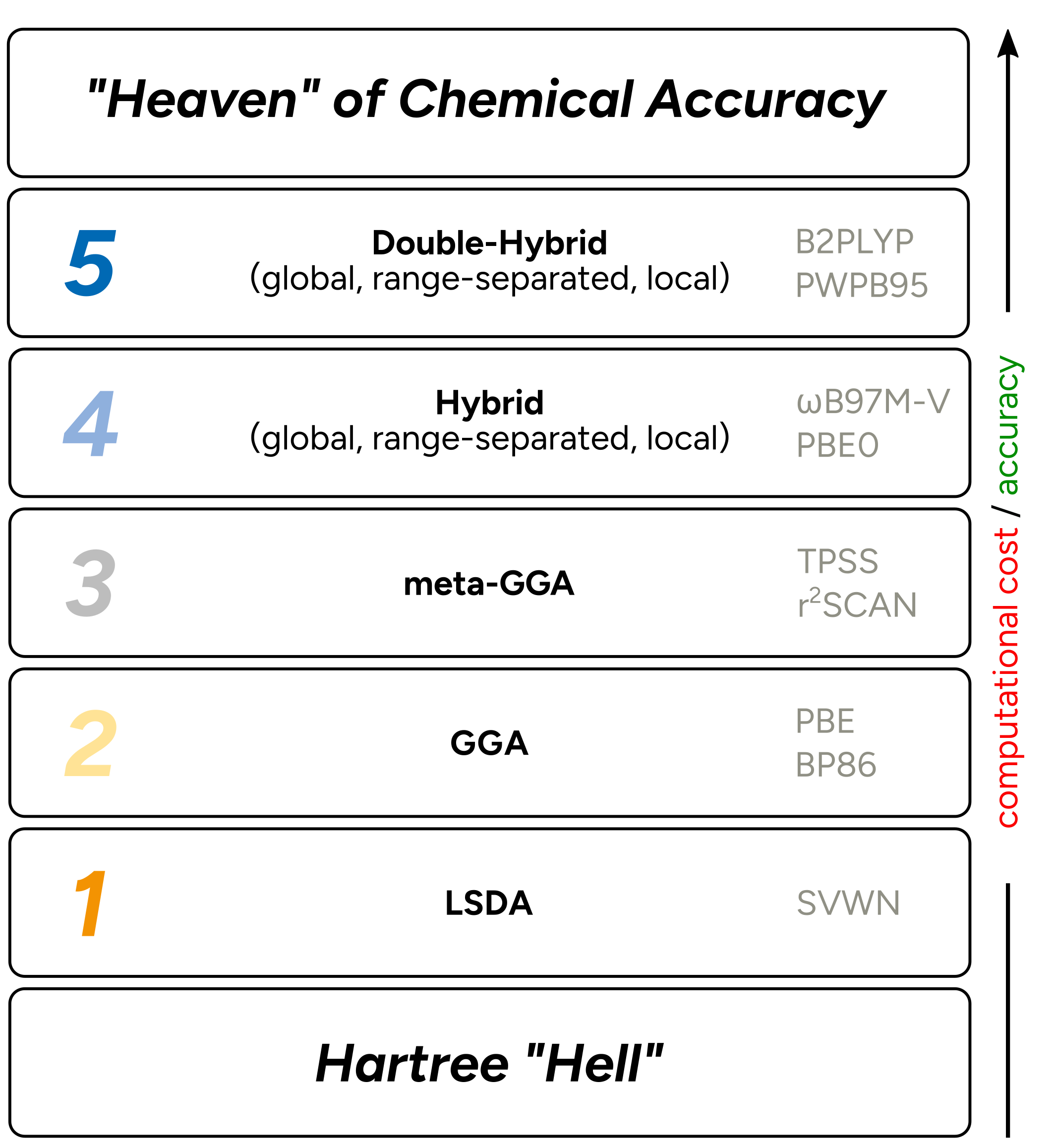
Fig. 3.1 Jacob’s ladder picture of density functionals.

ORCA features various density functionals of each rung either implemented natively or via the LibXC Functional Library. These functionals can be combined with various basis sets and relativistic approaches. Further, ORCA features a useful toolkit of resolution-of-identity (RI) methods to speed-up DFT calculations.

For dispersion corrections that can be used with DFT and the respective available functional-specific parameters refer to the Dispersion Corrections section.

Also note that some functionals like the SCAN and Minnesota families may require enhanced numerical integration grid settings.

3.4.1. Basic Usage

All implemented DFT methods can be invoked via their respective keywords, e.g. !PBE using the simple input line:

! PBE

Warning

If only a functional is defined, various default settings will be used including a small def2-SVP basis set, an appropriate RI treatment and default numerical integration grids! To achieve higher accuracy, specifically the basis set should be adjusted!

Many functionals can also be invoked via the %method block even though double-hybrid functionals being not available due to technical reasons:

%method
   Method DFT        # equivalent to method DFGTO
   Functional PBE
end

ORCA further provides some more utility to construct and modify functionals via the %method block. These expert options are described in the respective sections of each functional rung. Various other functionals can also be invoked via the LibXC Functional Library.

3.4.2. Local Functionals

Local exchange-correlation functionals are the most basic examples of functionals constructed according to equation (3.1):

(3.1)\[E_{\text{XC} } = E_{\text{LSD} }^{\text{X} } + E_{\text{LSD} }^{\text{C} } \]

They typically the original Slater exchange functional with different local correlations functionals like VWN-V[196] or PW-LDA[197]. All available local functional that are available in ORCA can be found in Table 3.1.

Table 3.1 List of available local functionals.

Functional	Keywords	Description
HFS	HFS	Hartree–Fock–Slater Exchange only functional
LDA or LSD	LDA, LSD	Local density approximation (defaults to VWN5)
VWN-V [196]	VWN,VWN5	Vosko-Wilk-Nusair local density approx. parameter set “V”
VWN-III [196]	VWN3	Vosko-Wilk-Nusair local density approx. parameter set “III”
PW-LDA [197]	PWLDA	Perdew-Wang parameterization of LDA

3.4.3. Gradient Corrected Functionals: (meta-)GGAs

The next rung corresponds to gradient corrected functional of the generalized gradient approximation (GGA) and the meta-generalized gradient approximation (meta-GGA) types. A simplified exchange-correlation energy expression for these types of functionals is given in (3.2). (meta-)GGAs are specifically useful for geometry optimizations and screening purposes due to their comparably small computational cost.

(3.2)\[E_{\text{XC} } = E_{\text{LSD} }^{\text{X} } + E_{\text{GGA} }^{\text{X} } + E_{\text{LSD} }^{\text{C} } + E_{\text{GGA} }^{\text{C} } \]

Table 3.2 List of available (meta-)GGA functionals.

Functional	Keyword	Description
GGAs
BP86 [198, 199]	BP86	Becke ‘88 exchange and Perdew ‘86 correlation
BLYP [200]	BLYP	Becke ‘88 exchange and Lee-Yang-Parr correlation
OLYP [201]	OLYP	Handy’s “optimal” exchange and Lee-Yang-Parr correlation
GLYP [202]	GLYP	Gill’s ‘96 exchange and Lee-Yang-Parr correlation
XLYP [203]	XLYP	The Xu and Goddard exchange and Lee-Yang-Parr correlation
PW91 [204]	PW91	Perdew-Wang ‘91 GGA functional
mPWPW [205]	MPWPW	Modified PW exchange and PW correlation
mPWLYP [205]	MPWLYP	Modified PW exchange and LYP correlation
PBE [206]	PBE	Perdew-Burke-Erzerhoff GGA functional
RPBE [207]	RPBE	“Modified” PBE
revPBE [208]	REVPBE	“Revised” PBE
RPW86PBE [209]	RPW86PBE	PBE correlation with refitted Perdew ‘86 exchange
PWP [204]	PWP	Perdew-Wang ‘91 exchange and Perdew ‘86 correlation
composite
B97-3c [210]	B97-3C	Composite DFT method by Grimme et al.
meta-GGAs
B97M-V [211]	B97M-V	Head-Gordon’s DF B97M-V with VV10 nonlocal correlation
B97M-D3(BJ) [212]	B97M-D3BJ	Modified version of B97M-V with D3BJ correction by Najibi and Goerigk
B97M-D4 [213]	B97M-D4	Modified version of B97M-V with DFT-D4 correction by Najibi and Goerigk
SCAN [214]	SCANFUNC	Perdew’s SCAN functional
rSCAN [215]	RSCAN	Regularized SCAN functional
r²SCAN [216]	R2SCAN	Regularized and restored SCAN functional by Furness, Sun et al.
M06-L [217]	M06L	The Minnesota M06-L meta-GGA functional
TPSS [218]	TPSS	The TPSS meta-GGA functional
revTPSS [219, 220]	REVTPSS	Revised TPSS meta-GGA functional
composite
r²SCAN-3c [221]	R2SCAN-3C	Composite DFT method by Grimme et al.

3.4.3.1. Customization of Basic Functionals

Basic exchange-correlation functionals can also be constructed from their components via the %method block using the Exchange, Correlation, and LDAOpt keywords. These controle the exchange and correlation parts of the functional as well as the local part of the correlation functional, respectively. For example BP86 (!BP86) is constructed from Becke’s ‘88 exchange via X_BECKE and Perdew’s ‘86 correlation functional via C_P86. In ORCA, it further employs Perdew and Wang’s LDA reparameterization[197] PWLDA for the local part of the correlation functional via C_PWLDA:

%method
   Method DFT
   Exchange     X_BECKE
   Correlation  C_P86
   LDAOpt       C_PWLDA
end

For a full list of available components see Table 3.3.

The correct choice of the local part of the correlation functional is crucial to ensure reproducibility of the results. In ORCA, almost all functionals choose PWLDA[197] as the underlying LDA functional as it represents a slightly better fit to the uniform electron gas than VWN. For VWN (Vosko, Wilk, and Nusair[196]), several parameterizations exist. In their classic paper give two sets of parameters – one in the main body (parametrization of RPA results; known as VWN-III) and one in their table 5 of correlation energies (parametrization of the Ceperley/Alder Monte Carlo results; known as VWN-V). The results from PW-LDA are very similar to those of VWN-V, whereas VWN-III yields quite different values. Over the years, the usage of different parameterizations for the same functional name throughout different quantum chemistry programs caused some confusion and deviating results. A prominent example is the different implementation of the B3LYP hybrid functional within ORCA and Gaussian. While ORCA uses VNW-V consistent with the TURBOMOLE program[222, 223, 224], the Gaussian program[225] employs VWN-III. Using the LDAOpt keyword, both variants can be constructed:

# consistent with TURBOMOLE
%method
   Method DFT
   Functional B3LYP
   LDAOpt C_VWN5
end

# consistent with Gaussian
%method
   Method DFT
   Functional B3LYP
   LDAOpt C_VWN3
end

For convenience both functionals can be invoked separately via the simple input keywords !B3LYP for the ORCA/TURBOMOLE variant and !B3LYP/G for the Gaussian variant.

Note

A special situation arises if LYP is the correlation functional [226] since LYP is not a correction to the correlation, but rather includes the full correlation. It is therefore used in the B3LYP functional as:

(3.3)\[E_{\text{B3LYP} }^{\text{C} } =E_{\text{LSD} }^{\text{C} } +c\left({ E_{\text{LYP} }^{\text{C} } -E_{\text{LSD} }^{\text{C} } } \right)\]

Some functionals further incorporate empirical parameters that can be changed to improve agreement with experiment. Currently, there are a few parameters that can be changed (other than the parameters used in the hybrid functionals, which are described later).

The first of these parameters is \(\alpha\) of Slater’s X\(_{\alpha }\) method. Theoretically, it has a value of 2/3 and this is used in the HFS and LSD functionals. However, the exchange contribution is underestimated by about 10% by this approximation (quite significant!) and a value around 0.70-0.75 is recommended for molecules.

The second parameter is the \(\beta\) for Becke’s gradient-corrected exchange functional. Becke determined the value 0.0042 by fitting the exchange energies for rare gas atoms. There is some evidence that with smaller basis sets, a slightly smaller value such as 0.0039 gives improved results for molecules.

The next parameter is the value \(\kappa\), which occurs in the PBE exchange functional. It has been given the value 0.804 by Perdew et al. in order to satisfy the Lieb-Oxford bound. Since then, other workers have argued that a larger value for this parameter (around 1.2) gives better energetics, which is explored in the revPBE functional. Note, however, that while revPBE gives slightly better energetics, it also gives slightly poorer geometries.

The last two parameters are also related to PBE. Within the PBE correlation functional, there is \(\beta_C\) (not to be confused with the \(\beta\) exchange parameter in Becke’s exchange functional), whose original value is \(\beta_C=0.066725\). Modified variants exist with different \(\beta_C\) values, e.g., the PBEsol functional and the PBEh-3c composite method. Furthermore, the \(\mu\) parameter in the PBE exchange functional may be modified. In the original formulation, it is related to \(\beta_C\) via \(\mu = \beta_C \frac{\pi^{2} }{3}\), but has been modified in later variants as well.

Table 3.3 %method block input keywords to modify basic exchange-correlation functionals.

Keyword	Options	Description
Exchange	X_NOX	No exchange
	X_SLATER	Slater’s local exchange
	X_BECKE	Becke’s ‘88 exchange
	X_wB88	Short-range Becke ‘88 exchange for range-separated functionals
	X_G96	Gill ‘96 gradient exchange
	X_PW91	Perdew-Wang (PW) ‘91 gradient exchange
	X_mPW	Adamo-Barone modification of PW exchange
	X_PBE	Perdew-Burke-Ernzerhof (PBE) exchange
	X_RPBE	Revised PBE exchange
	X_OPTX	Hoe/Cohen/Handy’s optimized exchange
	X_X	Xu/Goddard exchange
	X_TPSS	TPSS meta-GGA exchange
	X_B97D	Grimme’s modified exchange for the B97-D GGA
	X_B97BECKE	Becke’s original exchange for the B97 hybrid
	X_SCAN	Perdew’s constrained exchange for the SCAN meta-GGA
	X_RSCAN	Perdew’s constrained exchange for the rSCAN meta-GGA
	X_R2SCAN	Perdew’s constrained exchange for the r²SCAN meta-GGA
Correlation	C_NOC	No correlation
	C_VWN5	Local Vosko-Wilk-Nusair correlation (parameter set “V”)
	C_VWN3	Local Vosko-Wilk-Nusair correlation (parameter set “III”)
	C_PWLDA	Local PW correlation
	C_P86	Perdew ‘86 correlation
	C_PW91	PW ‘91 correlation
	C_PBE	PBE correlation
	C_LYP	LYP correlation
	C_TPSS	TPSS meta-GGA correlation
	C_B97D	Grimme’s modified correlation for the B97-D GGA
	C_B97BECKE	Becke’s original correlation for the B97 hybrid
	C_SCAN	Perdew’s constrained correlation for the SCAN meta-GGA
	C_RSCAN	Perdew’s constrained correlation for the rSCAN meta-GGA
	C_R2SCAN	Perdew’s constrained correlation for the r²SCAN meta-GGA
LDAOpt	C_NOC	Sets the local part of any correlation functional to no correlation
	C_PWLDA	Sets the local part of any correlation functional to PWLDA
	C_VWN5	Sets the local part of any correlation functional to VWN5
	C_VWN3	Sets the local part of any correlation functional to VWN3
Specific Parameters
XAlpha	<real>	Modifies Slater’s \(\alpha\) parameter (default 2/3)
XBeta	<real>	Modifies Becke’s \(\beta\) parameter (default 0.0042)
XKappa	<real>	Modifies the PBE(exchange) \(\kappa\) parameter (default 0.804)
XMuePBE	<real>	Modifies the PBE(exchange) \(\kappa\) parameter (default 0.21952)
CBetaPBE	<real>	Modifies the PBE(correlation) beta parameter (default 0.066725)

3.4.4. Hybrid DFT

The idea of replacing a portion of the DFT exchange by exact exchange from Hartree-Fock theory (HFX) was introduced by Becke in 1993[227, 228]. This scheme is typically referred to as hybrid DFT and the most simple formulation of a one-parameter hybrid functional is depicted in equation (3.4)

(3.4)\[E_{\text{hyb}}^{\text{XC}} =aE_{\text{HF}}^{\text{X}} + (1-a){ E_{\text{GGA}}^{\text{X}}} + E_{\text{GGA}}^{\text{C}}\]

A more general description is given by the adiabatic connection model (ACM). In the ACM, hybrid functionals are constructed with three parameters according to equation (3.5):

(3.5)\[E_{\text{XC} } = a E_{\text{HF} }^{\text{X} } +\left( 1 - a \right)E_{\text{LSD} }^{\text{X} } +bE_{\text{GGA} }^{\text{X} } +E_{\text{LSD} }^{\text{C} } +cE_{\text{GGA} }^{\text{C} } \]

Here, \(E_{\text{XC} }\) is the total exchange/correlation energy, \(E_{\text{HF} }^{\text{X} }\) is the Hartree-Fock exchange, \(E_{\text{LSD} }^{\text{X} }\) is the local (Slater) exchange, \(E_{\text{GGA} }^{\text{X} }\) is the gradient correction to the exchange, \(E_{\text{LSD} }^{\text{C} }\) is the local, spin-density based part of the correlation energy, and \(E_{\text{GGA} }^{\text{C} }\) is the gradient correction to the correlation energy.

Over the years, various strategies to construct hybrid functionals have been developed. These range from physics motivated approaches relying on as few as possible parameters like the overall well-balanced PBE0 functional[229] to more empirical variants like the prominent three-parameter hybrid B3LYP[230]. Furthermore, various treatments of the HF exchange admixture were developed. The basic hybrids that use a static amount of HFX are typically referred to as global hybrids while functionals with variable amounts of HFX include range-separated hybrids and local hybrids. Various global and range-separated hybrid functionals are available in ORCA. Local hybrids may be implemented in a future version.

ORCA also provides a sophisticated infrastructure to create and customize global and range-separated hybrid functionals.

Note

As by theory hybrid functionals are significantly more costly than (meta-)GGAs, ORCA uses the sophisticated RIJCOSX algorithm as a default to speed up hybrid DFT calculations.

3.4.4.1. Global Hybrid Functionals

Global hybrid functionals employ a fixed amount of Hartree-Fock exact exchange. ORCA features various representatives with different compositions and amounts of HFX. The optimal amount of HFX is controversially discussed in the literature and many empirical functionals were constructed by fitting it to reproduce an experimental property. However, it has been argued from a theoretical viewpoint that the optimal mixing of HF exchange is 25% [231] and large amounts of HFX are known to be disadvantageous for transition metal complexes.

A list of natively implemented global hybrid functionals is given in Table 3.4.

Table 3.4 List of available global hybrid functionals.

Functional	Keyword	%HFX	Description
hybrid GGAs
B1LYP [232]	B1LYP	25	The one-parameter hybrid functional with Becke ‘88 exchange and Lee-Yang-Parr correlation (25% HF exchange)
B3LYP [230]	B3LYP	20	The popular B3LYP functional (20% HF exchange) as defined in the TurboMole program system (LDAOPT C_VWN5)
B3LYP/G [230]	B3LYP/G	20	The popular B3LYP functional (20% HF exchange) as defined in the Gaussian program system (LDAOPT C_VWN3)
O3LYP [233]	O3LYP	11.61	The Handy hybrid functional
X3LYP [203]	X3LYP	21.8	The Xu and Goddard hybrid functional
B1P86 [199]	B1P86	25	The one-parameter hybrid version of BP86
B3P86 [227]	B3P86	20	The three-parameter hybrid version of BP86
B3PW91 [227]	B3PW91	20	The three-parameter hybrid version of PW91
PW1PW [229]	PW1PW	25	One-parameter hybrid version of PW91
mPW1PW [205]	MPW1PW	25	One-parameter hybrid version of mPWPW
mPW1LYP [205]	MPW1LYP	25	One-parameter hybrid version of mPWLYP
PBE0 [229]	PBE0	25	One-parameter hybrid version of PBE
revPBE0 [234]	REVPBE0	25	“Revised” PBE0
revPBE38 [234]	REVPBE38	37.5	“Revised” PBE0 with 37.5% HF exchange
BHandHLYP [227]	BHANDHLYP	50	Half-and-half hybrid functional by Becke
hybrid meta-GGAs
TPSSh [218]	TPSSH	10	The hybrid version of TPSS (10% HF exchange)
TPSS0 [235]	TPSS0	25	A 25% exchange version of TPSSh that yields improved energetics
r²SCANh [236]	R2SCANH	10	Global hybrid variant of r²SCAN with 10% HF exchange
r²SCAN0 [236]	R2SCAN0	25	Global hybrid variant of r²SCAN with 25% HF exchange
r²SCAN50 [236]	R2SCAN50	50	Global hybrid variant of r²SCAN with 50% HF exchange
composite
PBEh-3c [237]	PBEH-3C	42	Composite DFT approach by Grimme et al.
B3LYP-3c [238]	B3LYP-3C	20	Composite DFT approach by Grimme et al.

3.4.4.1.1. Customization of Global Hybrids

Global hybrid functional parameters can be customized via the %method block. For the customization of the basic exchange and correlation components see the Customization of Basic Functionals section. The important parameters for hybrid functionals are those used in the ACM model (cf. equation (3.5)). In this case, we will recreate the PBE0 functional (25% HFX) by using the ACM syntax:

! RIJCOSX
# PBE0
%method
   Method DFT
   Functional PBE
   ACM_A        0.25      # fraction of Hartree-Fock exchange
   ACM_B        0.75      # fraction of the GGA exchange
   ACM_C        1.00      # fraction of the GGA correlation
   ScalLDAC     1.00      # fraction of LDA correlation, must be equal to ACM_C 
end

For simplicity, the ACM parameters can also be given as one string.

! RIJCOSX
# PBE0
%method
   Method DFT
   Functional PBE
   ACM       0.25, 1.00, 1.00   # as ACM   ACM-A, ACM-B, ACM-C
   ScalLDAC  1.00               # fraction of LDA correlation, must be equal to ACM_C 
end

As the ACM formalism can be non-intutive, ORCA provides an equivalent syntax to control the respective parameters.

! RIJCOSX
# PBE0
%method
   Method DFT
   Functional PBE
   ScalHFX        0.25      # fraction of Hartree-Fock exchange
   ScalDFX        0.75      # fraction of GGA exchange
   ScalGGAC       1.00      # fraction of GGA correlation
   ScalLDAC       1.00      # fraction of LDA correlation, must be equal to ScalGGAC 
end

Warning

Note that Functional chooses specific predefined values for the variables Exchange, Correlation, LDAOpt and ACM described below. If given as a simple input keyword, in some cases, it will also activate a dispersion correction. You can explicitly give these variables instead or in addition to Functional. However, make sure that you specify these variables after you have assigned a value to Functional or the others will be reset to the values chosen by Functional.

Table 3.5 %method block input keywords to modify global hybrid functionals.

Keyword	Options	Description
ACM	<real, real, real>	Defines the ACM-A, ACM-B, and ACM-C parameters
ACM_A	<real>	Defines the ACM-A parameter (fraction of Hartree-Fock exchange)
ACM_B	<real>	Defines the ACM-B parameter (fraction of GGA exchange)
ACM_C	<real>	Defines the ACM-C parameter (fraction of GGA correlation)
ScalHFX	<real>	Controls the fraction of Hartree-Fock exchange, equiv. to ACM_A
ScalDFX	<real>	Controls the fraction of GGA exchange, equiv. to ACM_B
ScalGGAC	<real>	Controls the fraction of GGA correlation, equiv. to ACM_C

3.4.4.2. Range-Separated Hybrid Functionals

Unlike global hybrids, range-separated hybrid (RSH) split the two-electron operator used for the exchange into a short-range (SR) and a long-range (LR) regime wherein the short-range part is typically described by DFT exchange and the long-range part by Hartree-Fock exchange. In ORCA, all range-separated hybrids use the error function splitting approach by Hirao and coworkers to distinguish both regimes (cf. equation (3.6)).[239] This allows the definition of DFT functionals that dominate the short-range part by an adapted exchange functional of LDA, GGA or meta-GGA level and the long-range part by Hartree-Fock exchange.

(3.6)\[r_{12}^{-1} = \underbrace{\text{erfc}(\mu \cdot r_{12}) \cdot r_{12}^{-1} }_{\text{SR} } + \underbrace{\text{erf}(\mu \cdot r_{12}) \cdot r_{12}^{-1} }_{\text{LR} }\]

where \(\text{erf}(x) = \frac{2}{\sqrt{\pi} } \int_{0}^{x} \exp(-t^{2}) dt\) and \(\text{erfc}(x) = 1 - \text{erf}(x)\). Note that the splitting is only applied to the exchange contribution; all other contributions (one-electron parts of the Hamiltonian, the electron-electron Coulomb interaction and the approximation for the DFT correlation) are not affected. Later, Handy and coworkers[240] generalized the ansatz to:

(3.7)\[r_{12}^{-1} = \underbrace{\frac{1 - [ \alpha + \beta \cdot \text{erf}(\mu \cdot r_{12})]}{ r_{12} }}_{\text{SR} } + \underbrace{\frac{\alpha + \beta \cdot \text{erf}(\mu \cdot r_{12}) }{r_{12} }}_{\text{LR} }\]

This form of the splitting used in ORCA is shown visually (according to Handy and coworkers) in Fig. 3.2.

Fig. 3.2 Graphical description of the range-separation ansatz. The gray area corresponds to Hartree-Fock exchange. \(\alpha\) and \(\beta\) follow Handy’s terminology [240].

Important

Currently, RSH functionals can be used for integral-direct single-point calculations, calculations involving the first nuclear gradient (i.e. geometry optimizations), frequency calculations, TDDFT, TDDFT nuclear gradient, and EPR/NMR calculations. As with the global hybrids, RIJCOSX is used by default to drastically speed up the calculations. Alternatively, only RIJONX can be used.

A list of available range-separated hybrid functionals is given in Table 3.6

Table 3.6 List of available range-separated hybrid functionals. \(\mu\) is the range-separation parameter.

Functional	Keyword	%HFX	\(\mu\) / \(\text{bohr}^{-1}\)	% fixed DFX
hybrid GGAs
\(\omega\)B97 [241]	WB97	0 – 100	0.40	—
\(\omega\)B97X [241]	WB97X	15.7706 – 100	0.30	—
\(\omega\)B97X-V [242]	WB97X-V	16.7 – 100	0.30	—
\(\omega\)B97X-D3 [243]	WB97X-D3	19.5728 – 100	0.25	—
\(\omega\)B97X-D3(BJ) [212]	WB97X-D3BJ	16.7 – 100	0.30	—
\(\omega\)B97X-D4 [213]	WB97X-D4	16.7 – 100	0.30	—
\(\omega\)B97X-D4rev[49]	WB97X-D4REV	16.7 – 100	0.30	—
CAM-B3LYP [240]	CAM-B3LYP	19 – 65	0.33	35%
LC-BLYP [244]	LC-BLYP	0 – 100	0.33	—
LC-PBE [239]	LC-PBE	0 – 100	0.47	—
hybrid meta-GGAs
\(\omega\)B97M-V [245]	WB97M-V	15 – 100	0.30	—
\(\omega\)B97M-D3(BJ) [212]	WB97M-D3BJ	15 – 100	0.30	—
\(\omega\)B97M-D4 [213]	WB97M-D4	15 – 100	0.30	—
\(\omega\)B97M-D4rev [49]	WB97M-D4REV	15 – 100	0.30	—
\(\omega\)r²SCAN [246]	WR2SCAN	0 – 100	0.30	—
composite
\(\omega\)B97X-3c [49]	WB97X-3C	16.7 – 100	0.30	—

3.4.4.2.1. Customizing Range-Separated Hybrids

Range-separated hybrid functional parameters can also be customized via the %method block. For the customization of the basic exchange and correlation components see the Customization of Basic Functionals section. Basic hybrid-related keywords and the respective ACM model are described in the Hybrid DFT and Customization of Global Hybrids sections.

In this example, we will recreate the LC-PBE functional:

! RIJCOSX
# LC-PBE
%method
   Method DFT
   Exchange X_LRCPBE
   Correlation C_PBE
   LDAOpt C_PWLDA
   ACM_A        0.00   # fraction of static Hartree-Fock exchange
   ACM_B        0.00   # fraction of static GGA exchange
   ACM_C        1.00   # fraction of GGA correlation
   ScalLDAC     1.00   # fraction of LDA correlation, must be equal to ScalGGAC 
   RangeSepEXX  true   # activates range-separated exchange
   RangeSepMu   0.47   # range-separation parameter, should be >0
   RangeSepScal 1.00   # fraction of variable HFX, should sum to 1 with ACM-A and ACM-B
end

Which is equivalent to the ScalX syntax described before.

! RIJCOSX
# LC-PBE
%method
   Method DFT
   Exchange X_LRCPBE
   Correlation C_PBE
   LDAOpt C_PWLDA
   ScalHFX      0.00   # fraction of static Hartree-Fock exchange
   ScalDFX      0.00   # fraction of static GGA exchange
   ScalGGAC     1.00   # fraction of GGA correlation
   ScalLDAC     1.00   # fraction of LDA correlation, must be equal to ScalGGAC 
   RangeSepEXX  true   # activates range-separated exchange
   RangeSepMu   0.47   # range-separation parameter, should be >0
   RangeSepScal 1.00   # fraction of variable HFX, should sum to 1 with ScalHFX and ScalDFX
end

Warning

The amount of fixed DFT Exchange (ACM_B or ScalDFX) can only be changed for CAM-B3LYP and LC-BLYP. Accordingly, ACM-B is ignored by the \(\omega\)B97 approaches as no corresponding \(\mu\)-independent exchange functional has been defined. While it is technically possible to choose an exchange functional that has no \(\mu\)-dependence, this makes no sense conceptually.

Table 3.7 %method block input keywords to modify range-separated hybrid functionals.

Keyword	Options	Description
RangeSepEXX	true	Activates range-separated exchange
RangeSepMu	<real>	Controls the range-separation parameter, should be >0
RangeSepScal	<real>	Controls the fraction of variable Hartree-Fock exchange

3.4.5. Double-Hybrid DFT

In addition to mixing the HF-exchange into a given density functional, Grimme has proposed to mix in a fraction of the MP2 correlation energy as calculated with hybrid DFT orbitals [247]. Such functionals may be referred to as “double-“hybrid functionals. The original expression by Grimme is:

(3.8)\[E_{\text{XC}} = aE_{\text{X}}^{\text{HF}} +\left({1-a} \right)E_{\text{X}}^{\text{DFT}} +\left({1-c} \right)E_{\text{C}}^{\text{DFT}} +cE_{\text{C}}^{\text{MP2}} \]

The first proposed double-hybrid functional by Grimme was B2PLYP.[247] This double-hybrid functional utilizes the B88 exchange functional and the LYP correlation functionals. It introduces 53% of Hartree-Fock exchange (\(a = 0.53\)) and replaces 27% of the DFT correlation energy by MP2 correlation energy (\(c = 0.27\)). Since then many other DH-DFT approaches that deviate from the original theme were developed. For example Grimme proposed DH functionals like PWPB95[248] that use spin-component-scaled MP2. Further, functionals whose composition was empirically fitted against databases without any physical constraints or restrictions as previously proposed in (3.8) like Martin’s DSD (dispersion corrected, spin-component scaled double-hybrid) functionals[249, 250, 251] were developed and refined with revDSD-PBEP86-D4[252] being one of the most well known representatives. Functionals of the XYG\(n\) family[253] or Head-Gordon’s \(\omega\)B97M(2)[254] employ differently constructed densities for the DFT and the perturbation-theory parts with the latter also basing on a range-separated hybrid functional. In principle, other correlated methods like dRPA or higher order MP theory may be used within the double hybrid scheme. However, the most common approach employs classical MP2 or its spin-component-scaled variants. The DLPNO approximation to MP2 is also available within ORCA and can be used to massively speed up the energy and gradient calculations for large systems. The accuracy and efficiency of DLPNO-DHs was extensively studied by Bursch, Neese and co-workers[255]. Common to almost all double-hybrid functionals is a comparably large amount of Hartree-Fock exchange of 50% and more. Most classical double-hybrid functionals following the scheme by Grimme can be utilized for single point calculations, analytic gradients (and thus also geometry optimizations[256], relaxed scans, and transition state searches), dipole moments and other first order properties, magnetic second order properties (chemical shifts and g-tensors without the frozen core approximation in the MP2 part), as well as for numerical polarizabilities and frequencies.

Some double-hybrid functionals were further optimized for excited state applications and will make use of a Doubles Corrections to correct the singles-only excited states within the time-dependent DFT (TD-DFT) framework. Some of them, like SCS-PBE-QIDH only make use of spin-component-scaling for the CIS(D) component of the calculation. However, many of them have recently also been tested for ground-state properties.[257]

Note

ORCA employs the RIJCOSX and RI-MP2 by default. If this is not wanted, RI can be deactivated generally by using the !NORI keyword or if only the RI approximation of the MP2 part should be deactivated via the %mp2 block:

%mp2
   RI false
end

Indeed, there is hardly ever any reason to use conventional MP2.

Note

Note that per default no MP2 response density is calculated as its construction adds significant overhead. In this case, only the double-hybrid energy is correct. The computation of the MP2 response density that is consistent with first-order properties from analytic first-derivatives can be requested via the %mp2 density relaxed end statement in the %mp2 block. The considerably less costly unrelaxed (expectation value-like) density may instead requested by %mp2 density unrelaxed end. However, this is not recommended since the changes to the relaxed density are considerable in our experience and the unrelaxed density has a much weaker theoretical status than its relaxed counterpart.

3.4.5.1. Global Double-Hybrid Functionals

Global double-hybrid functionals are based on the respective global hybrid functionals and employ static admixtures of Hartree-Fock exchange and the MP2 correlation energy. A list of currently implemented global double-hybrid functionals is given in Table 3.8. The revDSD-PBEP86-D4[252] by Martin and co-workers has proven to be accurate for most thermochemistry applications.

Warning

For some functionals of the DSD/DOD family, different parameters for the same functional name were provided by the authors. The employed parameterization is indicated by the (year-of-publication) suffix of the functional and the respective keywords. Also not that for some of them, the basic parameters change in presence of different dispersion corrections. Please carefully check, if the employed parameters agree with your expectations!

Hint

For most natively implemented double-hybrids you can simple add the DLPNO- prefix to the respective functional simple input keyword, e.g. DLPNO-B2PLYP. For all others, the DLPNO treatment can be activated via the %mp2 block using the DLPNO true keyword.

Table 3.8 List of available global double-hybrid functionals. PS is the opposite-spin, PT the same-spin scaling parameter. Excited-states optimized functionals only employ spin-component-scaling for the CIS(D) doubles correction within the the TD-DFT framework. Same-spin indirect term (CTss), opposite-spin indirect term (CTos), same-spin direct term (CUss), and opposite-spin direct term (CUos) parameters are given in the footnotes.

Functional	Keywords	%HFX	%DFX	%GGAC	%MP2C	PS	PT
DSD-BLYP [249]	DSD-BLYP D3BJ	69	31	54	100	0.46	0.37
DSD-BLYP-NoDisp(2013) [251]	DSD-BLYP/2013	75	25	53	100	0.46	0.60
DSD-BLYP-D3(BJ)(2013) [251]	DSD-BLYP/2013 D3BJ	71	29	54	100	0.47	0.40
DSD-PBEP86 [250]	DSD-PBEP86 D3BJ	70	30	43	100	0.53	0.25
DSD-PBEP86-NoDisp(2013) [251]	DSD-PBEP86/2013	72	28	44	100	0.51	0.36
DSD-PBEP86-D3(BJ)(2013) [251]	DSD-PBEP86/2013 D3BJ	69	31	44	100	0.52	0.22
DSD-PBEB95-NoDisp [251]	DSD-PBEB95	70	30	52	100	0.48	0.22
DSD-PBEB95-D3(BJ) [251]	DSD-PBEB95 D3BJ	66	34	55	100	0.46	0.09
B2PLYP [247]	B2PLYP	53	47	73	27	–	–
mPW2PLYP [258]	mPW2PLYP	55	45	75	25	–	–
B2GP-PLYP [259]	B2GP-PLYP	65	35	64	36	–	–
B2K-PLYP [260]	B2K-PLYP	72	28	58	42	–	–
B2T-PLYP [260]	B2T-PLYP	60	40	69	31	–	–
B2NC-PLYP [261]	B2NC-PLYP	81	19	45	55	–	–
PWPB95 [248]	PWPB95	50	50	73.1	26.9	1.0	0.0
PBE-QIDH [262]	PBE-QIDH	69	31	67	33	–	–
PBE0-DH [263]	PBE0-DH	50	50	87.5	12.5	–	–
revDSD-PBEP86(2021) [252]	REVDSD-PBEP86/2021	69	31	42.24	100	0.5935	0.0566
revDSD-PBEP86-D4(2021) [252]	REVDSD-PBEP86-D4/2021	69	31	42.24	100	0.5935	0.0566
revDOD-PBEP86(2021) [252]	REVDOD-PBEP86/2021	69	31	43.01	100	0.6131	0.0
revDOD-PBEP86-D4(2021) [252]	REVDOD-PBEP86-D4/2021	69	31	43.01	100	0.6131	0.0
SOS1-r²SCAN-CIDH [246]	R2SCAN-CIDH	55	45	83.33	16.67	1.333	0.0
SOS1-r²SCAN-QIDH [246]	R2SCAN-QIDH	69.34	30.76	66.67	33.33	1.333	0.0
SOS1-r²SCAN0-2 [246]	R2SCAN0-2	79.37	20.63	50	50	1.333	0.0
SOS1-r²SCAN0-DH [246]	R2SCAN0-DH	50	50	87.50	12.50	1.333	0.0
Pr²SCAN50 [246]	PR2SCAN50	50	50	75	25	1.333	0.0
Pr²SCAN69 [246]	PR2SCAN69	69.34	30.76	55.56	44.44	1.333	0.0
\(\kappa\)Pr²SCAN50 [246]	KPR2SCAN	50	50	70	30	1.333	0.0
excited state opt.
SCS/SOS-B2PLYP21 [264]	SCS/SOS-B2PLYP21	53	47	73	27	[1]	[1]
SCS-PBE-QIDH [264]	SCS-PBE-QIDH	69	31	67	33	[2]	[2]
SOS-PBE-QIDH [264]	SOS-PBE-QIDH	69	31	67	33	[3]	[3]
SCS-B2GP-PLYP21 [264]	SCS-B2GP-PLYP21	65	35	64	36	[4]	[4]
SOS-B2GP-PLYP21 [264]	SOS-B2GP-PLYP21	65	35	64	36	[5]	[5]

3.4.5.2. Range-Separated Double-Hybrid Functionals

Range-separated double-hybrids employ variable amounts of Hartree-Fock exchange much like range-separated hybrid functionals and static amounts of MP2 correlation. A list of available range-separated double-hybrid functionals is given in Table 3.9.

Hint

For most natively implemented double-hybrids you can simple add the DLPNO- prefix to the respective functional simple input keyword, e.g. DLPNO-WPR2SCAN50. For all others, the DLPNO treatment can be activated via the %mp2 block using the DLPNO true keyword.

Table 3.9 List of available range-separated double-hybrid functionals. PS is the opposite-spin, PT the same-spin scaling parameter. \(\mu\) is the range-separation parameter. Excited-states optimized (ES-Opt.) functionals only employ spin-component-scaling for the CIS(D) doubles correction within the the TD-DFT framework. Same-spin indirect term (CTss), opposite-spin indirect term (CTos), same-spin direct term (CUss), and opposite-spin direct term (CUos) parameters are given in the footnotes.

Functional	Keywords	%HFX	\(\mu\) / \(\text{bohr}^{-1}\)	%GGAC	%MP2C	PS	PT
\(\omega\)B97M(2)[6] [254]	WB97M(2)	62.194 – 100	0.30	100	34.096	–	–
\(\omega\)B97X-2(TQZ) [265]	WB97X-2	63.6158 – 95.1661	0.30	100	100	0.447105	0.529319
\(\omega\)Pr2SCAN50 [246]	WPR2SCAN50	50 – 100	0.214013	65	35	1.333	0.000
RSX-QIDH [266]	RSX-QIDH	69 – 100	0.27	67	33	–	–
RSX-0DH [267]	RSX-0DH	50 – 100	0.33	87.5	12.5	–	–
\(\omega\)B2PLYP [268]	WB2PLYP	53 – 100	0.30	73	27	–	–
\(\omega\)B2GP-PLYP [268]	WB2GP-PLYP	65 – 100	0.27	64	36	–	–
\(\omega\)B88PP86 [268]	WB88PP86	65 – 100	0.20	58	42	–	–
\(\omega\)PBEPP86 [268]	WPBEPP86	70 – 100	0.18	68	48	–	–
excited state opt.
SCS/SOS-\(\omega\)B2PLYP [264]	SCS/SOS-WB2PLYP	53 – 100	0.30	73	27	[7]	[7]
SCS-\(\omega\)B2GP-PLYP [264]	SCS-WB2GP-PLYP	65 – 100	0.27	64	36	[8]	[8]
SOS-\(\omega\)B2GP-PLYP [264]	SOS-WB2GP-PLYP	65 – 100	0.27	64	36	[9]	[9]
SCS-RSX-QIDH [264]	SCS-RSX-QIDH	69 – 100	0.27	67	33	[10]	[10]
SOS-RSX-QIDH [264]	SOS-RSX-QIDH	69 – 100	0.27	67	33	[11]	[11]
SCS-\(\omega\)B88PP86 [264]	SCS-WB88PP86	65 – 100	0.20	58	42	[12]	[12]
SOS-\(\omega\)B88PP86 [264]	SOS-WB88PP86	65 – 100	0.20	58	42	[13]	[13]
SCS-\(\omega\)PBEPP86 [264]	SCS-WPBEPP86	70 – 100	0.18	68	48	[14]	[14]
SOS-\(\omega\)PBEPP86 [264]	SOS-WPBEPP86	70 – 100	0.18	68	48	[15]	[15]

3.4.5.2.1. \(\omega\)B97M(2)

Some double-hybrid functionals, such as \(\omega\)B97M(2)[254] must be applied to orbitals converged with a different functional. This can be accomplished with a two-step calculation using MORead and MaxIter=1. Note that because the orbitals are not obtained self-consistently, only single point energies can be computed in this way, i.e. no density, gradient, or properties! The usage of such functionals may be automatized using the Compound script language. An exemplary compound script for a \(\omega\)B97M(2) single-point calculation is given below:

*xyz 0 1
  H 0.0 0.0 0.0
  F 0.0 0.0 0.9
*
# ------------------------------------------------------------------------------------
# Energy calculation with the wB97M(2) double-hybrid functional, as defined in
# N. Mardirossian, M. Head-Gordon, J. Chem. Phys. 2018, 148, 241736.
# The final energy is calculated non-variatonally using wB97M-V orbitals.
# Note that FrozenCore is on default - one can turn it off using kw2 = "NoFrozenCore".
# Author: Georgi L. Stoychev
# ------------------------------------------------------------------------------------

# Optional variables:
Variable NLOpt = "SCNL";        # Consistent with Q-Chem. "NL" likely very similar. Only matters for Step 1.
Variable Basis = "def2-TZVP";   # Should be TZ or higher for reliable results
Variable AuxC  = "def2-TZVP/C"; # RI-MP2 is used by default. Must be compatible with the Basis
Variable AuxJ  = "def2/J";      # RIJCOSX is used by default
Variable RIMP2 = True;          # Set to false to turn off RI-MP2
Variable Grid  = "defGrid2";    # Should be OK.
Variable kw1   = "";            # Additional simple input keywords for step 1
Variable kw2   = "";            # Additional simple input keywords for step 2

# Output variables
Variable EwB97MV, EwB97M2;      # Will hold the final energies

# Step 1: wB97M-V calculation to obtain the orbitals
New_Step
  ! wB97M-V &{NLOpt} &{Grid} &{kw1}
  %basis
    Basis "&{Basis}"
    AuxJ  "&{AuxJ}"
  end
Step_End

# Step 2: single iteration with the wB97M(2) functional + MP2 correlation to get the final energy
ReadMOs(1);
New_Step
  ! wB97M(2) &{NLOpt} &{Grid} &{kw2} NoIter CalcGuessEnergy
  %basis
    Basis "&{Basis}"
    AuxC  "&{AuxC}"
    AuxJ  "&{AuxJ}"
  end
  %scf
    IgnoreConv 1
  end
  %mp2 RI &{RIMP2} end
Step_End

Read EwB97MV = DFT_Total_En[1];
Read EwB97M2 = MP2_Total_Energy[2];

Print("");
Print("================================================================================\n");
Print(" wB97M-V Energy:  %20.10lf\n",EwB97MV);
Print(" wB97M(2) Energy: %20.10lf\n",EwB97M2);

End

3.4.5.3. Customization of Double-Hybrids

As double-hybrid functionals make use of customizable components of global hybrids or range-separated hybrids they can can be constructed and customized in similar fashion. The MP2 correlation treatment for double-hybrids can be controlled via the DoMP2 true and ScalMP2C keywords within the %method block. Moreover, the MP2 treatment can be further customized via the %mp2 block. For example, the spin-composite-scaled, range-separated double-hybrid functional \(\omega\)Pr²SCAN50 can be constructed as follows:

! RIJCOSX def2-TZVP/C NOTRAH
# wPr2SCAN50
%method
   Method       DFT
   DoMP2        true       # activates MP2 correlation part
   Exchange     X_WR2SCAN
   Correlation  C_R2SCAN
   LDAOpt       C_PWLDA
   ScalHFX      0.50       # fraction of static Hartree-Fock exchange
   ScalDFX      0.00       # fraction of static GGA exchange
   ScalGGAC     0.65       # fraction of GGA correlation
   ScalLDAC     0.65       # fraction of LDA correlation, must be equal to ScalGGAC 
   ScalMP2C     0.35       # fraction of MP2 correlation
   RangeSepEXX  true       # activates range-separated exchange
   RangeSepMu   0.214013   # range-separation parameter, should be >0
   RangeSepScal 0.50       # fraction of variable HFX, should sum to 1 with ScalHFX and ScalDFX
end
%mp2
   DoSCS        true       # activates spin-component-scaling
   RI           true       # activate RI-MP2
   PS           1.333      # opposite-spin-scaling parameter
   PT           0.000      # same-spin-scaling parameter
end

Many other MP2 related options like the DLPNO treatment and ragularization can be found in the MP2 section of the manual.

Table 3.10 Most important %method block input keywords to customize double-hybrid functionals.

Keyword	Options	Description
DoMP2	true	Activates MP2 correlation part
ScalMP2C	<real>	Controls the fraction of GGA exchange

Table 3.11 Most important %mp2 block input keywords to customize double-hybrid functionals. For more details see the MP2 section.

Keyword	Options	Description
DoSCS	true	Activates spin-component-scaling of MP2 part
PS	<real>	Controls the opposite-spin-scaling parameter
PT	<real>	Controls the same-spin-scaling parameter
RI	true	Activates RI-MP2
DLPNO	true	Activates DLPNO-MP2

3.4.6. LibXC Functional Library

It is possible to use the functionals provided by LibXC within the ORCA framework [16]. The LibXC version used by ORCA is printed at the beginning of the output. The LibXC reference should be cited when LibXC is used as part of your calculations. For reference, see [269].

The complete list of functionals available via the LibXC interface can always be inspected by typing at the command line

orca -libxcfunctionals

The list of functionals has the following form:

Functionals available via LibXC:
  No.:     ID / Keyword                    - Name
    0:     18 / lda_c_1d_csc               - Casula, Sorella & Senatore
    1:     26 / lda_c_1d_loos              - P-F Loos correlation LDA
    2:     15 / lda_c_2d_amgb              - AMGB (for 2D systems)
    3:     16 / lda_c_2d_prm               - PRM (for 2D systems)
    4:    552 / lda_c_br78                 - Brual & Rothstein 78

   ...

The list is grouped by “level” of functional (LDA, GGA, meta-GGA, etc.) and then by part of the energy it models (correlation, exchange, exchange-correlation). Correlation functionals carry a ’_c_’ in their names, exchange functionals an ’_x_’, and combined exchange-correlation functionals an ’_xc_’. Additional information for a specific functional can be requested using

orca -libxcinfo [functional name]

where the functional name is the keyword in the above list.

Specification of LibXC functionals in the ORCA input follows the standard format:

%method 
  Method     DFT
  Functional hyb_gga_xc_b3lyp
end

or in the case of separate exchange and correlation specifications:

%method 
  Method      DFT
  Exchange    mgga_x_m06_l
  Correlation mgga_c_m06_l
end

CAM-type range-separated functionals are supported through the LibXC interface since ORCA 5.0. So are functionals that include non-local (VV10) correlation (see Non-Local Dispersion Correction (VV10): DFT-NL). The VV10 part is computed internally by ORCA. Other non-local functionals, such as BEEF-vdW, are not supported. Meta-GGA functionals that depend on the kinetic energy density \(\tau\) are supported, but not those that depend on the Laplacian of the density \(\nabla^2\rho\).

Double-hybrid functionals can be constructed with LibXC components as described in the previous customization sections, but only with separate exchange and correlation components. So exchange=gga_x_pbe and correlation=gga_c_pbe can be used, but functional=hyb_gga_xc_pbeh cannot be used in a double-hybrid formulation. Beware that the exchange and correlation contributions calculated by LibXC are simply scaled by ScalDFX and ScalGGAC, respectively, and no care is taken to separately scale LDA components or alter other internal parameters!

3.4.6.1. Screening Thresholds

When the density is smaller than a certain threshold, LibXC skips the evaluation of the functional and instead sets all the output quantities to zero in order to avoid under- and/or overflows. The default thresholds for different functionals are set by the LibXC developers, but may sometimes be too low. We have not performed extensive testing, but allow the user to set the threshold. Similarly, there are thresholds for minimum values of \(\zeta\) and \(\tau\) in order to avoid division by zero. The default values are functional-independent and can be changed using the following keywords.

%method 
  LibXCDensityThreshold 1e-12    # seems to be reasonable
  LibXCZetaThreshold    2e-16    # default value in LibXC
  LibXCTauThreshold     1e-20    # default value in LibXC
end

3.4.6.2. Modifying LibXC Functional Parameters

Starting with ORCA 5.1 it is possible to modify the “external parameters” of a functional that the LibXC interface provides. The available parameters and their default values can be seen in the output or with the orca -libxcinfo command above. Please exercise caution when using this interface and if using a published functional reparametrization, make sure you can reproduce results from the original publication. The syntax requires one of the ExtParamX, ExtParamC, or ExtParamXC keywords (depending on which functional is modified), followed by the parameter name in quotation marks, and finally the new value. For example, here is an input for the PWPB95 double-hybrid functional, where the simple input keyword is used to set most parameters (such as the MP2 scaling factors) and only the exchange and correlation parameters of the mPW91 and B95 LibXC functionals, respectively, are modified.

! Opt PWPB95 def2-SVP def2-SVP/C

%method
  Exchange    gga_x_mpw91
  Correlation mgga_c_bc95
  ExtParamX   "_bt"     0.00444
  ExtParamX   "_alpha" 19.823391
  ExtParamX   "_expo"   3.7868
  ExtParamC   "_css"    0.03241
  ExtParamC   "_copp"   0.00250
end

*xyz 0 1
  H 0 0 0
  F 0 0 0.9
*

Note that the variable definitions in LibXC may be different from the ones used internally in ORCA or in the original publication, due to various constant factors, etc. When in doubt, please consult the LibXC documentation or source code repository — we simply provide access to the interface.

3.4.6.3. Simple Input of LibXC Functionals

Some LibXC functionals are accessible via the simple input keyword !LibXC(Keyword), e.g. !LibXC(TPSS). The keywords match those of the natively implemented in ORCA. Using this syntax, parameters for the DFT-D dispersion corrections are also set automatically (if implemented). Table Table 3.12 lists the available functionals and their LibXC names.

Table 3.12 LibXC functionals available via the simple input !LibXC(Keyword)

Keyword	LibXC components	Notes
GGAs
B97-D	gga_xc_b97_d	Uses D2
B97-D3	gga_xc_b97_d	Uses D3(0)
B97-D4	gga_xc_b97_d	Uses D4
BLYP	gga_x_b88 + gga_c_lyp
KT2	gga_xc_kt2
KT3	gga_xc_kt3
PBE	gga_x_pbe + gga_c_pbe
REVPBE	gga_x_pbe + gga_c_pbe	\(\kappa\)=1.245
XLYP	gga_xc_xlyp
meta-GGAs
B97M-V	mgga_xc_b97m_v	Uses VV10
B97M-D3BJ	mgga_xc_b97m_v	Uses D3(BJ)
B97M-D4	mgga_xc_b97m_v	Uses D4
M06L	mgga_x_m06_l + mgga_c_m06_l
MN15L	mgga_x_mn15_l + mgga_c_mn15_l
MTASK-LDA	mgga_x_mtask + lda_c_pw_mod
MTASK-SCAN	mgga_x_mtask + mgga_c_scan
REVTM	mgga_x_revtm + mgga_c_revtm
R2SCAN	mgga_x_r2scan + mgga_c_r2scan
RSCAN	mgga_x_rscan + mgga_c_rscan
SCAN	mgga_x_scan + mgga_c_scan
TASK-CCALDA	mgga_x_task + mgga_c_ccalda
TASK-CC	mgga_x_task + mgga_c_cc
TASK-LDA	mgga_x_task + lda_c_pw_mod
TASK-SCAN	mgga_x_task + mgga_c_scan
TM	mgga_x_tm + mgga_c_tm
TPSS	mgga_x_tpss + mgga_c_tpss
hybrid GGAs
B1PW	gga_x_b88,gga_c_pw91	Custom mixing
B1PBE	gga_x_b88 + gga_c_pbe	Custom mixing
B3PW91	hyb_gga_xc_b3pw91	Custom mixing
B3LYP	hyb_gga_xc_b3lyp5
B3LYP/G	hyb_gga_xc_b3lyp
B3LYPS	hyb_gga_xc_b3lyps	B3LYP*, 15% HFX
B97	hyb_gga_xc_b97
CAM-B3LYP	hyb_gga_xc_cam_b3lyp	Custom mixing
CASE21	hyb_gga_xc_case21
G1LYP	gga_x_g96 + gga_c_lyp	Custom mixing
HSE06	hyb_gga_xc_hse06
HSE12	hyb_gga_xc_hse12
HSE12S	hyb_gga_xc_hse12s
HSESOL	hyb_gga_xc_hse_sol
KMLYP	hyb_gga_xc_kmlyp
LB07	hyb_gga_xc_lb07
LC-BLYP	hyb_gga_xc_lc_blyp	Custom mixing
MPW1LYP	hyb_gga_xc_mpw1lyp	Custom mixing
MPW1PW	hyb_gga_xc_mpw1pw	Custom mixing
PBE0	hyb_gga_xc_pbeh
PBE38	hyb_gga_xc_pbe38
PBE50	hyb_gga_xc_pbe50
PW91_0	gga_x_pw91 + gga_c_pw91	Custom mixing
PW1PW	gga_x_pw91 + gga_c_pw91	Custom mixing
REVPBE0	gga_x_pbe,gga_c_pbe	\(\kappa\)=1.245
REVPBE38	gga_x_pbe,gga_c_pbe	37.5% HFX, \(\kappa\)=1.245
WHPBE0	hyb_gga_xc_whpbe0
WB97	hyb_gga_xc_wb97
WB97X	hyb_gga_xc_wb97x
WB97X-D3	hyb_gga_xc_wb97x_d3	Uses D3(0)
WB97X-V	hyb_gga_xc_wb97x_v	Uses VV10
WB97X-D3BJ	hyb_gga_xc_wb97x_v	Uses D3(BJ)
WB97X-D4	hyb_gga_xc_wb97x_v	Uses D4
WB97X-D4REV	hyb_gga_xc_wb97x_v	Uses D4 with revised parameters
hybrid meta-GGAs
GAS22	hyb_mgga_xc_gas22
M05	hyb_mgga_x_m05 + mgga_c_m05
M052X	hyb_mgga_x_m05_2x + mgga_c_m05_2x
M06	hyb_mgga_x_m06 + mgga_c_m06
M062X	hyb_mgga_x_m06_2x + mgga_c_m06_2x
M06SX	hyb_mgga_x_m06_sx + mgga_c_m06_sx
MN15	hyb_mgga_x_mn15 + mgga_c_mn15
LC-TMLYP	hyb_mgga_xc_lc_tmlyp
PW6B95	hyb_mgga_xc_pw6b95
R2SCANH	hyb_mgga_xc_r2scanh
R2SCAN0	hyb_mgga_xc_r2scan0
R2SCAN38	hyb_mgga_xc_r2scanh	37.5% HFX
R2SCAN50	hyb_mgga_xc_r2scan50
SCAN0	hyb_mgga_x_scan0 + mgga_c_scan
TPSS0	hyb_mgga_xc_tpss0
TPSSH	hyb_mgga_xc_tpssh
WB97M-V	hyb_mgga_xc_wb97m_v	Uses VV10
WB97M-D3BJ	hyb_mgga_xc_wb97m_v	Uses D3(BJ)
WB97M-D4	hyb_mgga_xc_wb97m_v	Uses D4
WB97M-D4REV	hyb_mgga_xc_wb97m_v	Uses D4 with revised parameters
double-hybrids
B2PLYP	gga_x_b88 + gga_c_lyp	Custom mixing
B2GP-PLYP	gga_x_b88 + gga_c_lyp	Custom mixing
B2T-PLYP	gga_x_b88 + gga_c_lyp	Custom mixing
B2K-PLYP	gga_x_b88 + gga_c_lyp	Custom mixing
B2NC-PLYP	gga_x_b88 + gga_c_lyp	Custom mixing
DSD-PBEB95-D3	gga_x_pbe + mgga_c_bc95	Custom mixing, uses D3(BJ)
DSD-PBEB95-D4	gga_x_pbe + mgga_c_bc95	Custom mixing, uses D4
MPW2-PLYP	gga_x_mpw91 + gga_c_lyp	Custom mixing
PWPB95	gga_x_mpw91 + mgga_c_bc95	Custom mixing and ExtParam’s
PBE0-DH	gga_x_pbe + gga_c_pbe	Custom mixing
PBE0-2	gga_x_pbe + gga_c_pbe	Custom mixing
PBE-QIDH	gga_x_pbe + gga_c_pbe	Custom mixing
PR2SCAN50	mgga_x_r2scan + mgga_c_r2scan	Custom mixing
PR2SCAN69	mgga_x_r2scan + mgga_c_r2scan	Custom mixing
SOS1-R2SCAN0-DH	mgga_x_r2scan + mgga_c_r2scan	Custom mixing
SOS1-R2SCAN-CIDH	mgga_x_r2scan + mgga_c_r2scan	Custom mixing
SOS1-R2SCAN-QIDH	mgga_x_r2scan + mgga_c_r2scan	Custom mixing
SOS1-R2SCAN0-2	mgga_x_r2scan + mgga_c_r2scan	Custom mixing

---

[1] (1,2)

SCS/SOS-B2PLYP21: CTss: 0.000; CTos: 0.334; CUss: 0.000; CUos: 0.283.

[2] (1,2)

SCS-PBE-QIDH: CTss: 0.070; CTos: 0.515; CUss: 0.096; CUos: 0.524.

[3] (1,2)

SOS-PBE-QIDH: CTss: 0.000; CTos: 0.547; CUss: 0.000; CUos: 0.573.

[4] (1,2)

SCS-B2GP-PLYP21: CTss: 0.018; CTos: 0.475; CUss: 0.000; CUos: 0.468.

[5] (1,2)

SOS-B2GP-PLYP21: CTss: 0.000; CTos: 0.489; CUss: 0.000; CUos: 0.484.

[6]

Must be used with ωB97M-V orbitals (cf. Section 3.4.5.2.1).

[7] (1,2)

SCS/SOS-\(\omega\)B2PLYP: CTss: 0.000; CTos: 0.433; CUss: 0.000; CUos: 0.460.

[8] (1,2)

SCS-\(\omega\)B2GP-PLYP: CTss: 0.000; CTos: 0.571; CUss: 0.135; CUos: 0.558.

[9] (1,2)

SOS-\(\omega\)B2GP-PLYP: CTss: 0.000; CTos: 0.570; CUss: 0.000; CUos: 0.610.

[10] (1,2)

SCS-RSX-QIDH: CTss: 0.174; CTos: 0.541; CUss: 0.586; CUos: 0.424.

[11] (1,2)

SOS-RSX-QIDH: CTss: 0.000; CTos: 0.632; CUss: 0.000; CUos: 0.714.

[12] (1,2)

SCS-\(\omega\)B88PP86: CTss: 0.000; CTos: 0.557; CUss: 0.092; CUos: 0.545.

[13] (1,2)

SOS-\(\omega\)B88PP86: CTss: 0.000; CTos: 0.559; CUss: 0.000; CUos: 0.599.

[14] (1,2)

SCS-\(\omega\)PBEPP86: CTss: 0.000; CTos: 0.610; CUss: 0.297; CUos: 0.540.

[15] (1,2)

SOS-\(\omega\)PBEPP86: CTss: 0.000; CTos: 0.613; CUss: 0.000; CUos: 0.669.

[16]

https://libxc.gitlab.io