Transition State Optimization¶

There are various ways to obtain a valid guess for a transition state (TS) structure like relaxed potential energy surface scans or NEB simulations. To only optimize a given transition state guess without using automated procedures like NEB-TS, the !OptTS keyword can be used. In the following tutorial, we will setup a relaxed surface scan to obtain a guess for the TS of the cis-trans-isomerization of glyoxal and subsequently optimize the transition state with !OptTS.

Example: cis-trans-Isomerization of Glyoxal¶

Relaxed Surface Scan¶

After obtaining a valid start structure for glyoxal with, e.g. Avogadro 2, a relaxed surface scan around the O-C-C-O dihedral angle can be setup using the !Opt simple keyword and the respective scan definition inside the %geom block. In this example, we will perform the scan with the r²SCAN-3c composite DFT method.

!r2SCAN-3c Opt

%geom
   Scan D 0 1 2 3  = 180, 360, 19 end # Scan of the dihedral angle defined by atoms 0, 1, 2, and 3 from 180° to 360° in 19 steps.
end

*xyz 0 1
  O          -1.80011949735812      0.99666410862853     -0.00003868102245
  C          -1.27328664864401     -0.08847334375096     -0.00001219100927
  C           0.24492627868679     -0.23050598341765     -0.00002272454655
  O           0.77147537164033     -1.31579795317196     -0.00003090426569
  H          -1.83500409491985     -1.04822924700392      0.00001280906050
  H           0.80714603899486      0.72893993091597     -0.00002459971653

Important

Note that ORCA starts counting atoms from 0, thus atom 1 has the identifier 0.

Tip

Make sure that the starting angle is not too far from that of your initial structure to avoid some artifacts.

After running this scan we obtain a smooth energy curve from which we can pick the structure with the highest energy as TS guess.

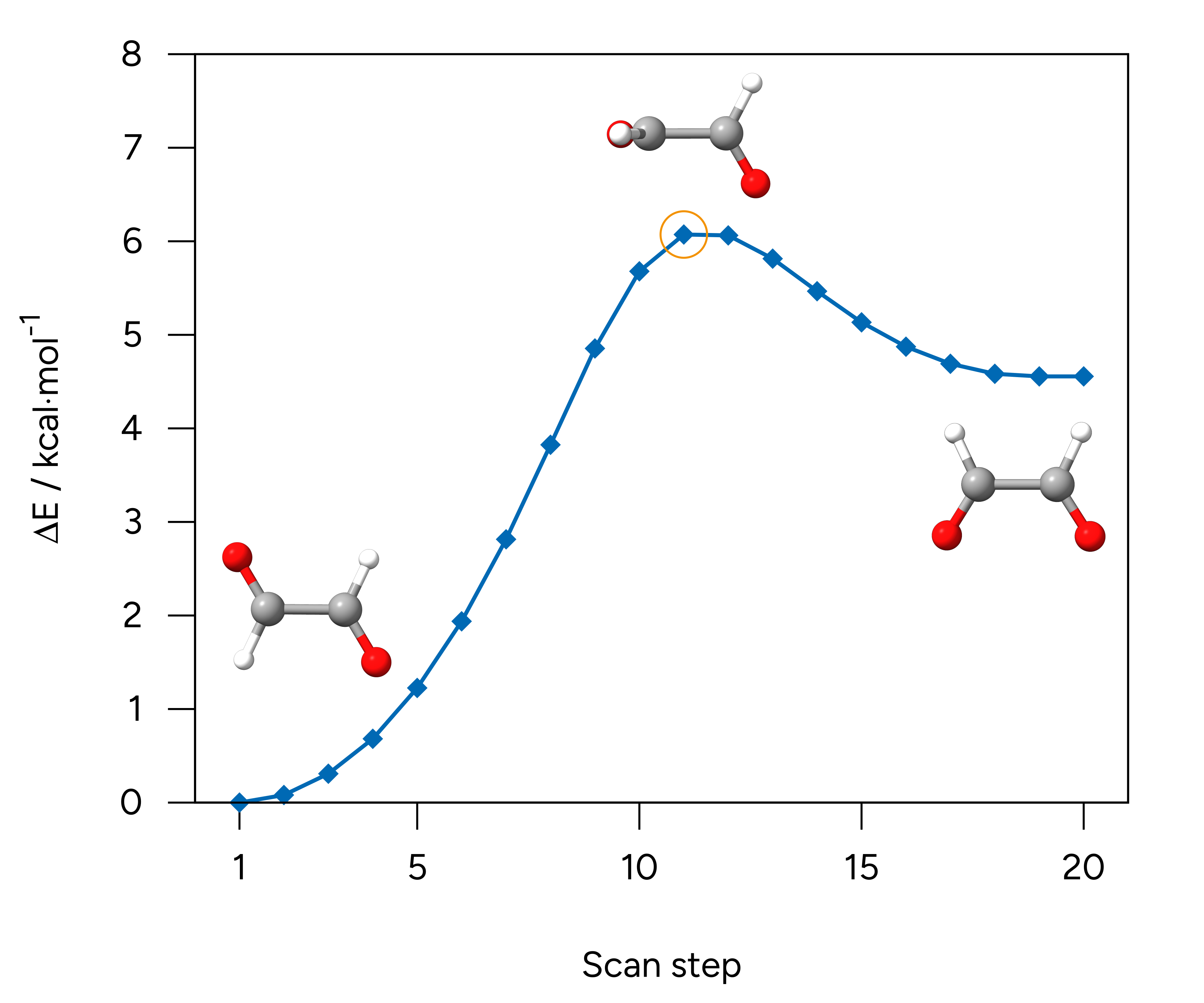
../_images/fig_scan.png — Figure: Relaxed scan of the O-C-C-O dihedral angle of glyoxal.¶

TS Optimization with `!OptTS`¶

The most common procedures starting from a TS guess are now:

Run a direct !OptTS calculation using a less accurate approximate Hessian (not recommended).
Run a direct !OptTS calculation requesting a prior exact Hessian calculation (recommended).
Run a exact Hessian calculation with !Freq, check the imaginary mode of the TS, and run !OptTS with reading the .hess file from the previous frequency calculation.

Warning

Using the approximate Hessian by simply running !OptTS can cause troubles with the TS localization. We generally recommend to use an exact Hessian to start the TS optimization.

Tip

By adding the !Freq simple input keyword aside !OptTS, a frequency calculation after the TS optimization is requested. This is useful to verify that the optimization yielded a transition state that is characterized by presence of exactly one imaginary frequency.

Tip

The transition state optimization can be customized in many ways to either improve efficiency or to handly difficult transition states, e.g., for very small barriers. Therefore, we recommend to read the respective sections of the ORCA manual. Note that the convergence thresholds for !OptTS are controlled by the existing keywords for normal optimizations like !TightOpt.

`!OptTS` with Approximate Hessian¶

An input for a TS optimization with approximate Hessian looks like

!r2SCAN-3c OptTS

*xyzfile 0 1 tsguess.xyz

The use of the approximate Almlöf Hessian is indicated in the .out file.

Evaluating the initial hessian          ...  (Almloef) done
[...]
Evaluating the initial hessian          ....  (Almloef) done

`!OptTS` with Exact Hessian¶

To calculate the exact Hessian for the TS optimization, the respective Calc_Hess true must be defined in the %geom block.

!r2SCAN-3c OptTS

%geom
   Calc_Hess true
end

*xyzfile 0 1 tsguess.xyz

The calculation of the exact Hessian prior the TS optimization is indicated in the .out file.

Evaluating the initial hessian          ...  (Is done on the fly) done
[...]
Evaluating the initial hessian          ....  (read)

`!OptTS` with Read-In Hessian¶

To read a previously computed Hessian, the inhess read keyword can be used within the %geom block, providing the name of the Hessian file via InHessName "name.hess".

!r2SCAN-3c OptTS

%geom
  inhess   Read                   # this command comes with:
  InHessName "tsguess.hess"       # filename of Hessian input file
end

*xyzfile 0 1 tsguess.xyz

If the .hess file has been read successfully, it is indicated in the .out file:

Evaluating the initial hessian          ... (Reading Exact Hessian)...
[...]
Evaluating the initial hessian          ....  (read)

TS Verification¶

As with conventional geometry optimizations, proper convergence must be achieved for the transition state optimization. TS optimization convergence is highlighted in the .out file. For this example, both options with exact and approximate Hessian worked and yield converged transition states with an O-C-C-O dihedral angle of ~75.5°.

                    ***********************HURRAY********************
                    ***        THE OPTIMIZATION HAS CONVERGED     ***
                    *************************************************

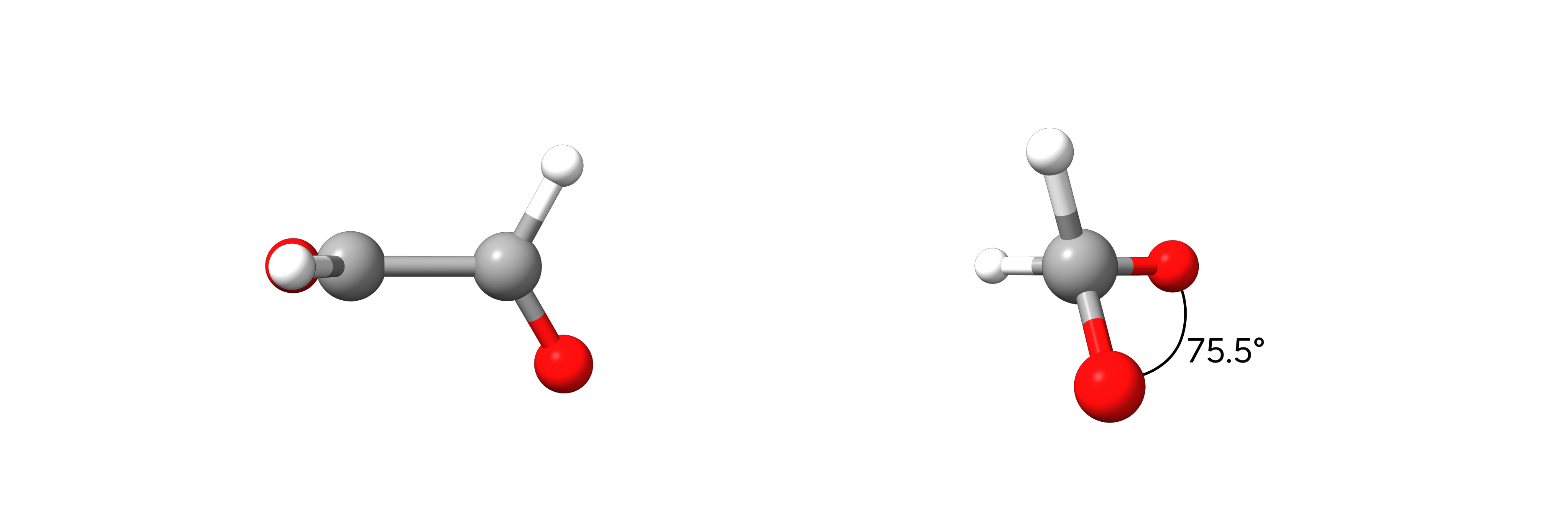
../_images/ts3.png — Figure: Optimized TS of the *cis*-*trans*-isomerization of glyoxal.¶

However, it is further important to check if the optimized structure is a minimum or a saddle point (TS) on the potential energy surface. The latter is characterized by exactly one imaginary frequency in the frequency calculations on the finally optimized TS geometry. This imaginary frequency must further represent the structural transition of interest, in this case the rotation around the C-C bond. Such frequency calculation is either requested by simply adding the !Freq simple input keyword aside !OptTS which requests a frequency calculation after the TS optimization. Alternatively, a separate calculation on the optimized geometry using !Freq can be performed.

Important

Note that the frequency calculation must be performed at the same level of theory as the geometry optimization!

A full input performing an exact Hessian calculation for the TS optimization input, the TS optimization, and subsequent frequency calculation for verification in one is given below.

!r2SCAN-3c OptTS Freq

%geom
   Calc_Hess true
end

*xyzfile 0 1 tsguess.xyz

For the optimized TS of the cis-trans-inversion of glyoxal, only one imaginary frequency corresponding to the rotation of the C-C bond is obtained, thus verifying a successful TS optimization for this example. The respective vibration can be visualized with various tools like Avogadro 2 or ChimeraX (cf. Graphical User Interfaces and the Infrared and Raman Spectroscopy sections).

-----------------------
VIBRATIONAL FREQUENCIES
-----------------------

Scaling factor for frequencies =  1.000000000  (already applied!)

     0:       0.00 cm**-1
     1:       0.00 cm**-1
     2:       0.00 cm**-1
     3:       0.00 cm**-1 
     4:       0.00 cm**-1
     5:       0.00 cm**-1
     6:    -189.59 cm**-1  ***imaginary mode***  
     7:     277.42 cm**-1

Transition State Optimization¶

Example: cis-trans-Isomerization of Glyoxal¶

Relaxed Surface Scan¶

TS Optimization with !OptTS¶

!OptTS with Approximate Hessian¶

!OptTS with Exact Hessian¶

!OptTS with Read-In Hessian¶

TS Verification¶

Structures¶

TS Optimization with `!OptTS`¶

`!OptTS` with Approximate Hessian¶

`!OptTS` with Exact Hessian¶

`!OptTS` with Read-In Hessian¶