ORCA with External Methods
Even though ORCA features a vast amount of electronic structure models, it cannot cover all available methods. Therefore, ORCA features an interface to external methods that allows you to use ORCA's optimization infrastructure with electronic structure methods and model potentials provided by external programs. This way you'll be able to utilize the latest MNDO based semi-empirical methods like PM7 or neural network potentials like AIMNet2 and UMA within the ORCA infrastructure, e.g. to optimize structures, search transition states with NEB-TS, or sample conformers with GOAT.
The external methods infrastructure can be accessed via the ORCA simple input keyword !ExtOpt which can be combined with other common keywords
like !Opt or !GOAT. As every program typically provides output in different formatting and style, individual wrapper scripts are required to link ORCA and its external optimizer infrastructure. The full path to your wrapper script can be provided via the %method block:
! ExtOpt

%method
  ProgExt "/full/path/to/wrapperscript"
  Ext_Params "optional command line arguments"
end
The Ext_Params keyword is used to set program specific options like methods, models, or solvation. A detailed list of available options per wrapper script is obtained by calling the respective script with the -h flag, e.g., oet_mopac -h.
Important
Some wrapper scripts and how to use them can be found in our ORCA-External-Tools GitHub repository. The repository is open to the community and contributions are very welcome!
Note
Note that depending on your OS and infrastructure, you may need to do some modifications to the wrapper script!
Note
In case of methods that are imported via Python interfaces such as AIMNet2 and UMA, two different scripts can be used. One is a standalone which might slow down your calculation due to heavy imports. The other option is a server/client approach. Here, the server must be started beforehand with the respective script and then the client script can be used similar to the other scripts. More information is given in the following examples or in the respective README files on GitHub.
Official wrapper scripts
The ORCA-External-Tools GitHub repository provides several ready-to-use scripts for programs like MOPAC and g-xTB, as well as neural network potentials like AIMNet2 and UMA. It also includes a framework that enables the quick implementation of new methods.
Installation
The repository contains an install.py that simplifies the installation process. Running it will create a virtual environment, by default called .venv, whose path should not be changed afterward. Additionally, a folder (by default called bin) will be created containing all executable scripts that can be used with ORCA. These scripts can be moved elsewhere if desired.
You can customize both the virtual environment path and the scripts directory during installation:
python install.py --venv-dir <path/to/venv/dir/> --script-dir <path/to/script/dir/>
If you want to use Python-based methods like AIMNet2, UMA, or MLatom you can add the -e flag to install the required dependencies:
python install.py -e aimnet2
python install.py -e uma
python install.py -e mlatom
Because these packages may have incompatible dependencies, it is recommended to create separate installations for each by specifying distinct virtual environment and script directories.
Note
If you maintain multiple environments, remember to set the script path explicitly during installation. Otherwise, the process may overwrite existing scripts.
Example 1: Optimization of Disorazol Z1 with PM7 via MOPAC
In this example, we will optimize disorazol, a potential anti-cancer drug, within ORCA utilizing energies and gradients generated with the PM7 method in MOPAC. To do so, we simply add the !Opt simple input keyword and an additional --method PM7 argument for the mopac wrapper script:
!ExtOpt Opt PAL4

%method
  ProgExt "/full/path/to/oet_mopac"
  Ext_Params "--method PM7"
end

*XYZFILE 0 1 structure.xyz
We can now run the ORCA input file via orca basename.inp as usual and the external optimizer infrastructure will generate two output files, the
normal ORCA output basename.out and the output of the external program, in this case MOPAC basename_EXT.out.
We can now check the ORCA output for convergence and will find the typical success message:
                    ***********************HURRAY********************
                    ***        THE OPTIMIZATION HAS CONVERGED     ***
                    *************************************************
The MOPAC output also indicates normal execution for the last energy and gradient calculation:
 **                              MOPAC v22.0.6                                **
 **                                                                           **
 *******************************************************************************
 **          Digital Object Identifier (DOI): 10.5281/zenodo.6511958          **
 **    Visit the DOI location for information on how to cite this program.    **
 *******************************************************************************

                              PM7 CALCULATION RESULTS

 *******************************************************************************
[...]
 **********************
 *                    *
 * JOB ENDED NORMALLY *
 *                    *
 **********************


 TOTAL JOB TIME:             0.62 SECONDS
The PM7 optimized structure is stored in the basename.xyz file as usual alongside the optimization trajectory basename_trj.xyz. The full optimization
of disorazol is shown in the animation below.
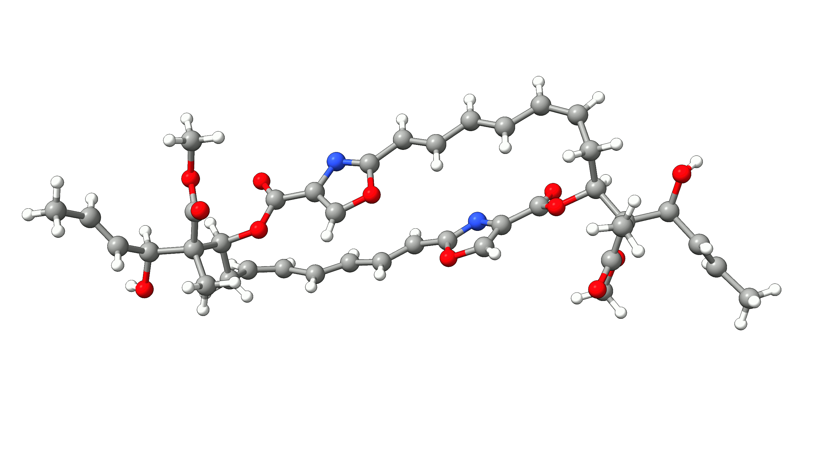
Figure: PM7 optimization of Disorazol Z1 using MOPAC via ORCA's external optimization feature.
Structures Example 1
Disorazol Z1 unoptimized
100

N      4.9056000000    9.4983000000    7.3808000000
N      3.7927000000    9.5666000000    2.0870000000
O      2.5573000000    8.0061000000    9.6644000000
O      3.3918000000   10.1213000000    9.7156000000
O      5.2191000000    7.4378000000    6.5692000000
O      8.0703000000    5.7271000000   -3.3425000000
H      8.4793000000    6.2292000000   -3.8777000000
O      3.8441000000    5.1815000000   -1.7983000000
O      4.1962000000    7.2585000000   -2.5227000000
O      5.7494000000    7.3570000000    0.0202000000
O      5.2928000000    9.5498000000   -0.3412000000
O      3.6351000000    7.8654000000    3.5190000000
O      0.1414000000    7.9363000000   13.2750000000
H     -0.0323000000    8.6062000000   13.7510000000
O      4.0052000000    5.9237000000   11.4984000000
O      4.1148000000    8.0439000000   12.1910000000
C      3.3498000000    8.9937000000    9.2481000000
C      4.1739000000    8.5676000000    8.1215000000
C      4.3556000000    7.3413000000    7.6276000000
H      3.9560000000    6.5429000000    7.9526000000
C      5.5061000000    8.8068000000    6.4792000000
C      6.3252000000    9.2591000000    5.4169000000
H      6.5409000000   10.1837000000    5.4085000000
C      6.8332000000    8.5052000000    4.4092000000
H      6.6774000000    7.5688000000    4.4252000000
C      7.5931000000    9.0500000000    3.3203000000
H      7.8827000000    9.9519000000    3.3933000000
C      7.9255000000    8.3786000000    2.2042000000
H      7.7777000000    7.4397000000    2.1753000000
C      8.5004000000    9.0299000000    1.0416000000
H      8.8888000000    9.8850000000    1.1815000000
C      8.5398000000    8.5555000000   -0.1902000000
H      8.9178000000    9.1235000000   -0.8513000000
C      8.0489000000    7.2107000000   -0.6584000000
H      8.1052000000    6.5656000000    0.0899000000
H      8.6358000000    6.8860000000   -1.3861000000
C      6.6079000000    7.2710000000   -1.1634000000
H      6.4818000000    8.0841000000   -1.7324000000
C      5.2131000000    8.5454000000    0.3262000000
C      4.4832000000    8.4751000000    1.5970000000
C      4.3950000000    7.4418000000    2.4632000000
H      4.7866000000    6.5835000000    2.3585000000
C      3.3035000000    9.1646000000    3.2191000000
C      2.4956000000    9.8742000000    4.1681000000
H      2.2882000000   10.7844000000    3.9959000000
C      2.0219000000    9.3133000000    5.2824000000
H      2.2487000000    8.4039000000    5.4406000000
C      1.2003000000    9.9627000000    6.2618000000
H      0.9438000000   10.8630000000    6.1060000000
C      0.7753000000    9.3696000000    7.3810000000
H      0.9868000000    8.4509000000    7.4986000000
C      0.0240000000   10.0149000000    8.4197000000
H     -0.3403000000   10.8681000000    8.2161000000
C     -0.2125000000    9.5385000000    9.6375000000
H     -0.7177000000   10.0976000000   10.2172000000
C      0.2270000000    8.2198000000   10.1989000000
H      0.1913000000    7.5389000000    9.4817000000
H     -0.4077000000    7.9461000000   10.9073000000
C      1.6423000000    8.2499000000   10.7851000000
H      1.8236000000    9.1522000000   11.1746000000
C      6.1247000000    6.0246000000   -1.9217000000
C      6.6730000000    6.0246000000   -3.3852000000
H      6.5642000000    6.9461000000   -3.7573000000
C      5.9542000000    5.0738000000   -4.2858000000
H      5.9810000000    4.1520000000   -4.0589000000
C      5.2885000000    5.4115000000   -5.3651000000
H      5.2418000000    6.3378000000   -5.5673000000
C      4.6049000000    4.4908000000   -6.2970000000
H      5.0371000000    4.5342000000   -7.1759000000
H      3.6641000000    4.7510000000   -6.3828000000
H      4.6600000000    3.5747000000   -5.9519000000
C      6.4819000000    4.7200000000   -1.1795000000
H      6.0961000000    3.9561000000   -1.6578000000
H      6.1195000000    4.7517000000   -0.2694000000
H      7.4560000000    4.6222000000   -1.1401000000
C      4.6014000000    6.0628000000   -2.0557000000
C      2.7629000000    7.3715000000   -2.6880000000
H      2.4485000000    6.6708000000   -3.2971000000
H      2.5461000000    8.2509000000   -3.0626000000
H      2.3245000000    7.2694000000   -1.8182000000
C      1.9499000000    7.1463000000   11.8547000000
C      1.5515000000    7.7172000000   13.2595000000
H      2.0156000000    8.5920000000   13.3965000000
C      1.9293000000    6.7865000000   14.3766000000
H      1.4671000000    5.9586000000   14.4302000000
C      2.8297000000    7.0217000000   15.2686000000
H      3.3353000000    7.8210000000   15.1781000000
C      3.1467000000    6.1272000000   16.4504000000
H      2.6361000000    5.2941000000   16.3758000000
H      2.9036000000    6.5858000000   17.2819000000
H      4.1052000000    5.9236000000   16.4580000000
C      1.2577000000    5.8417000000   11.5618000000
H      0.2911000000    5.9489000000   11.6841000000
H      1.5894000000    5.1510000000   12.1728000000
H      1.4415000000    5.5743000000   10.6365000000
C      3.4517000000    6.9453000000   11.8293000000
C      5.5498000000    7.9725000000   12.1232000000
H      5.8177000000    7.5826000000   11.2654000000
H      5.8841000000    7.4133000000   12.8554000000
H      5.9258000000    8.8744000000   12.2038000000
Example 2: NEB-TS with PM6-D3H4X via MOPAC
In this example, we will run a NEB-TS transition state search of the dihydrogen activation by Erker's frustrated Lewis pair (FLP) within ORCA utilizing energies and gradients generated with the PM6-D3H4X method in MOPAC. PM6-D3H4X is the default method chosen in the wrapper script. Therefore, no further method definition is required.

Figure: Dihydrogen activation by Erker's frustrated Lewis pair.
The corresponding ORCA input includes the full path to the MOPAC wrapper mopac.py and the usual NEB-TS input:
!ExtOpt NEB-TS PAL8

%method
  ProgExt "/full/path/to/oet_mopac"
end

%NEB
  NEB_END_XYZFILE "products.xyz"
  PreOpt true
  NImages 15
END

*XYZFILE 0 1 reactants.xyz
To link ORCA and MOPAC, we will use the mopac.py wrapper script that is available in our ORCA-External-Tools GitHub repository. The full path to that script must be defined via the progext keyword in the %method block.
We can now run the ORCA input file as usual via orca basename.inp > basename.out and if everything is set up properly, ORCA will call MOPAC via the wrapper script to calculate energies and gradients and reformat them to be readable by ORCA. The ORCA output will look the same as if the chosen task, in this case
NEB-TS was done with any method native to ORCA.
After the successful NEB-TS run, the generated minimum energy pathway is stored as basename_MEP_trj.xyz and can be visualized using one of various
graphical user interfaces and the relative energies can be plotted.
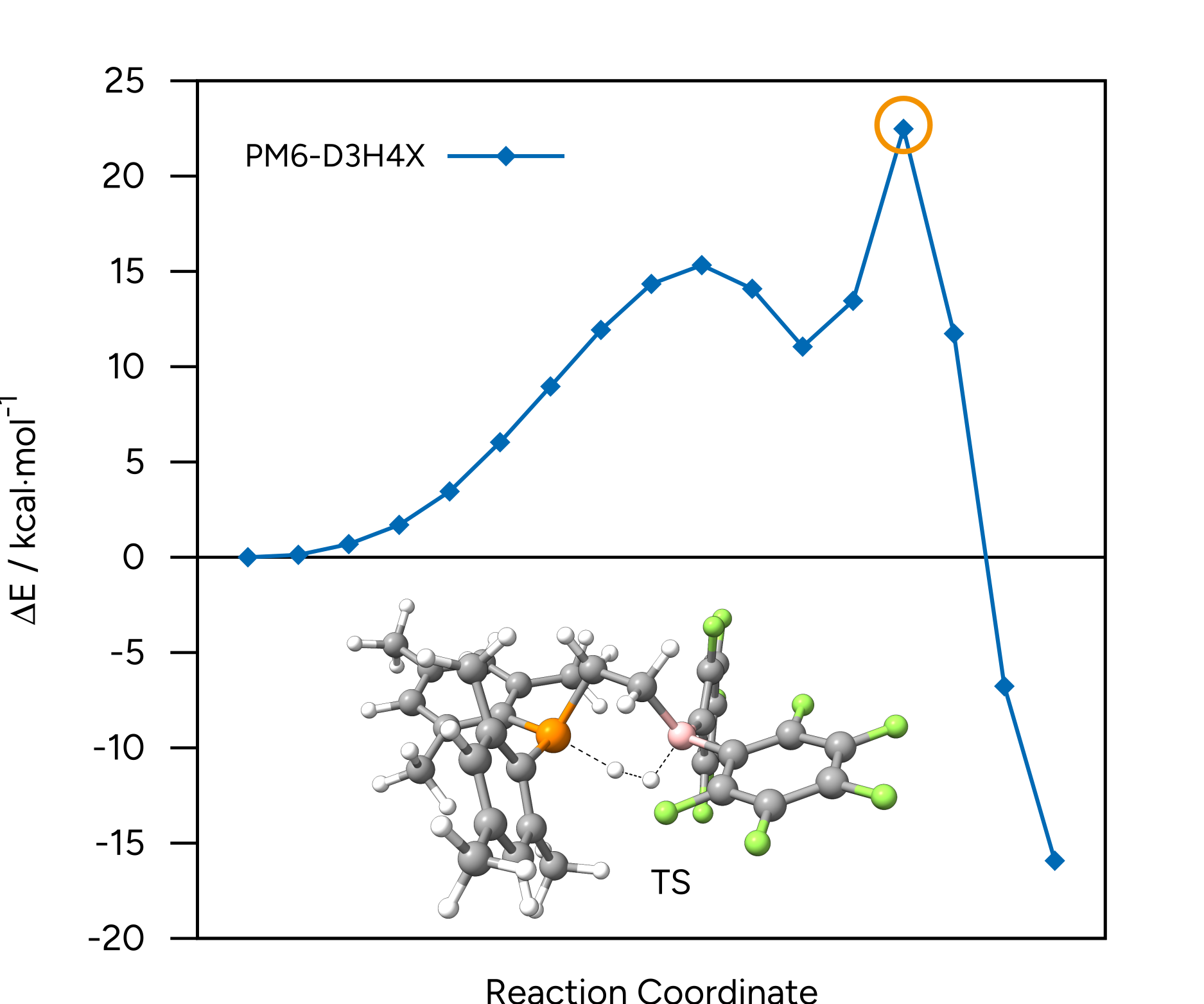
Figure: NEB-TS minimum energy path and TS guess at the PM6-D3H4X level.
Structures Example 2
Reactants
72

P     -0.3662186668   -0.4096435953    2.4180808260
H     -2.3885845963    2.9955626038    5.4479529454
C      3.5664000355   -1.2461611941    0.0460721904
C      4.0345311647   -2.4799363070   -0.4218846155
C      0.5906956936    0.2741158964    0.9024119146
C      3.5926063693   -0.9405728379    1.4305609924
C      4.5295774292   -3.4308472274    0.4683424173
C      4.5577094567   -3.1556020395    1.8335312075
C      4.0922904559   -1.9282805675    2.3166260030
F      3.1102486338   -0.3601181140   -0.8720376588
F      4.0021101028   -2.7560478584   -1.7496868199
F      4.9741403016   -4.6268853216    0.0074899162
F      1.6609927682    2.4069841606    3.8673812046
C     -0.7759877333    0.8592881293    5.2072930505
C     -1.4939909110    1.0603727091    2.7564911367
C     -2.3065451624    1.7164461694    1.7700735919
C     -3.0879214210    2.8224332432    2.1412495307
C     -3.1135208398    3.2836385061    3.4572948761
C     -2.3445997439    2.6407919742    4.4247654087
C     -1.5404447670    1.5392172532    4.0953319641
C     -2.4846728629    1.2620308898    0.3401290842
H     -3.7127028087    3.3080989098    1.3989223051
C     -3.9915180710    4.4386702859    3.8472359970
C     -3.7015934076   -0.9976824375    2.7817835838
C     -1.4544914791   -1.7959121031    1.7030713575
C     -0.8119512656   -2.8653235985    0.9961802904
C     -1.5662737058   -3.8866609251    0.4051153805
C     -2.9470678924   -3.9294813072    0.5367618161
C     -3.5865139050   -2.9635810366    1.3034699798
C     -2.8773777715   -1.9059311104    1.9015453922
C      0.6819036932   -3.0332378272    0.8715721201
H     -1.0640870808   -4.6743923886   -0.1457984450
C     -3.7492527548   -5.0276088777   -0.0971420363
H     -4.6599624638   -3.0451075440    1.4349647467
B      3.0131350631    0.4514405801    2.0128430573
C      5.5998693277    1.5036915913    4.7858506455
F      5.0250895074   -4.0897589233    2.6989572953
C      3.6623672934    1.1516096769    3.3212470857
C      1.7990587780    1.1803087417    1.2101586227
C      3.5424989674    2.6717065465    5.2406955397
C      2.9450043758    2.0748303851    4.1243326081
F      5.8097090173    0.0955408361    2.9136274998
C      4.8629985399    2.3837814910    5.5735623559
C      5.0154824347    0.8944206734    3.6702979916
F      6.8964470055    1.2469203924    5.0950886633
F      5.4364357513    2.9702372312    6.6536309660
F      2.8327779615    3.5384554667    6.0062750205
F      4.0918640768   -1.7367717031    3.6606716382
H      0.9522007858   -0.5586335520    0.2878715846
H     -0.0387216445    0.8519353506    0.2211678560
H      1.4521972827    2.1118638057    1.6812212976
H      2.2187472490    1.5065174227    0.2373150753
H      1.2597087595   -2.3232278677    1.4806724365
H      0.9682076828   -4.0312044561    1.2673758660
H      0.9898144936   -2.9734141085   -0.1934005127
H     -4.7345601984   -1.3813207626    2.9216722406
H     -3.2485998390   -0.9334458836    3.7925050715
H     -3.8598668324   -0.0135626474    2.3409536060
H     -3.1033972147   -5.7316587228   -0.6633823322
H     -4.2901809290   -5.5978503546    0.6870174798
H     -4.4867829971   -4.5870722156   -0.8009478600
H     -2.0262115947    0.2848534207    0.1168859802
H     -3.5663902937    1.1076816015    0.1403115110
H     -2.1084885857    2.0393134711   -0.3581158096
H     -4.5580195499    4.8362082252    2.9777413749
H     -4.7247988658    4.1041275923    4.6121757931
H     -3.3732792824    5.2572015006    4.2701561221
H     -0.9351373579    1.3585919087    6.1869438451
H     -1.1222854849   -0.1908963403    5.3037483428
H      0.3093227895    0.8512713219    5.0034519911
H      0.7540838587   -2.8519089197    4.2554242046
H      1.2874419057   -3.0099218389    4.6931723926
Product
72

P     -0.5141474859   -0.6146687557    1.7732495131
H     -2.3073527307    2.5415227122    5.2483856969
C      3.8976464054   -0.7736830433    0.6748291330
C      4.5247100662   -1.8426146794    0.0226708706
C      0.7960404084    0.5055582004    1.0062180750
C      3.4852219019   -0.9019184371    2.0229276441
C      4.7715428862   -3.0366122778    0.7012890616
C      4.3956596054   -3.1689505522    2.0378517298
C      3.7562694931   -2.1149435235    2.6966389400
F      3.7084071929    0.3775089920   -0.0174764085
F      4.9014355568   -1.7168802815   -1.2745115723
F      5.3877541089   -4.0650705258    0.0663580708
F      1.9047854228    2.1938758994    4.8731094145
C     -0.8427860787    0.3354249557    4.7853059771
C     -1.5308898507    0.8388913102    2.3740198414
C     -2.2590127333    1.6544577280    1.4587108400
C     -2.9713968215    2.7670210580    1.9330673660
C     -2.9841209658    3.0889912371    3.2918457138
C     -2.2844527789    2.2872147662    4.1946961177
C     -1.5588624833    1.1681184778    3.7562781608
C     -2.3425715705    1.3777010917   -0.0222948677
H     -3.5255341394    3.3828669768    1.2340679650
C     -3.7470530146    4.2814694178    3.7931113692
C     -3.8558392207   -0.9993416846    2.6178364960
C     -1.7438745807   -2.0168792915    1.4681251655
C     -1.2013404525   -3.1504470909    0.7739207164
C     -2.0139939380   -4.2447116719    0.4577087755
C     -3.3567024222   -4.2709212780    0.8086780201
C     -3.9001692448   -3.1972478291    1.5078030549
C     -3.1289717182   -2.0686592584    1.8469557506
C      0.2403947588   -3.2805834797    0.3178390294
H     -1.5914867403   -5.0883136780   -0.0793534987
C     -4.2188629803   -5.4446818188    0.4453839376
H     -4.9485595045   -3.2468255157    1.7801953312
B      2.7567394502    0.2837013655    2.8476373452
C      6.0177199541    1.8502977606    4.4413803101
F      4.6541406446   -4.3233386945    2.7015593213
C      3.7762991086    1.1673199976    3.7398485466
C      1.7418275425    1.2332396443    1.9746652311
C      4.0864550469    2.8327398877    5.5034165123
C      3.2433615125    2.0637578055    4.6968703954
F      5.7852925983    0.2434250342    2.7363841220
C      5.4699451414    2.7266087992    5.3767201544
C      5.1875367204    1.0730681512    3.6253815578
F      7.3653983211    1.7491256408    4.3236838833
F      6.2823210744    3.4726519303    6.1657947726
F      3.5558807405    3.6825160121    6.4180585237
F      3.4137698580   -2.2805742554    4.0010234345
H      1.3905441557   -0.1307651185    0.3307470817
H      0.3053046121    1.2541114761    0.3556310926
H      1.1294752714    1.8711165172    2.6397637822
H      2.3805453331    1.9199621863    1.3802760347
H      0.9033881401   -2.4347594800    0.5565380917
H      0.6932355562   -4.1780305532    0.7913133181
H      0.2691623290   -3.4079172290   -0.7846856501
H     -4.9025534621   -1.2872244579    2.8533990521
H     -3.3562237151   -0.8243962839    3.5890394907
H     -3.9449201055   -0.0828962455    2.0185058970
H     -3.6461985220   -6.2183222471   -0.1091328387
H     -4.6347687204   -5.9073257277    1.3660122938
H     -5.0549875324   -5.1032784554   -0.2011287679
H     -1.8025143116    0.4663469530   -0.3375470978
H     -3.4070932679    1.2362719138   -0.3068286369
H     -1.9328360358    2.2409662666   -0.5876555927
H     -4.2561256215    4.8200797514    2.9652184492
H     -4.5167210280    3.9535666366    4.5231508839
H     -3.0505409799    4.9872577739    4.2928544539
H     -0.9872448071    0.7306319616    5.8138247919
H     -1.2220341262   -0.7066181096    4.7622904255
H      0.2361316733    0.3321254109    4.5832569326
H      0.3630550367   -1.4428985924    2.5800866384
H      2.0804831254   -0.2794083001    3.6378813047
Example 3: GOAT with AIMNet2
In this example, we will use GOAT to generate a conformer ensemble for the anti-inflammatory drug ibuprofen. For this, we want to use AIMNet2 with the server/client scripts available in our ORCA-External-Tools GitHub repository.
We first have to start the AIMNet2 server by executing the oet_server script:
oet_server aimnet2 --nthreads 4
When the server is running, we can use the oet_client client via ORCA input:
! EXTOPT GOAT PAL8

%method
  ProgExt "/full/path/to/oet_client"
end

*XYZfile 0 1 ibuprofen.xyz
Note
Once the server is initialized with aimnet2, it can handle different models/parameterizations. If not already present, the selected model will be installed in the .venv directory. Depending on your download speed, this might take a few minutes.
We can now run the ORCA input file as usual via orca basename.inp > basename.out and if everything is set up properly, ORCA will call AIMNet2 via the wrapper script to calculate energies and gradients and reformat them to be readable by ORCA.
After the successful GOAT run, the final conformer ensemble is stored in basename.finalensemble.xyz that can be visualized with graphical user interfaces
like Avogadro 2 or ChimeraX.
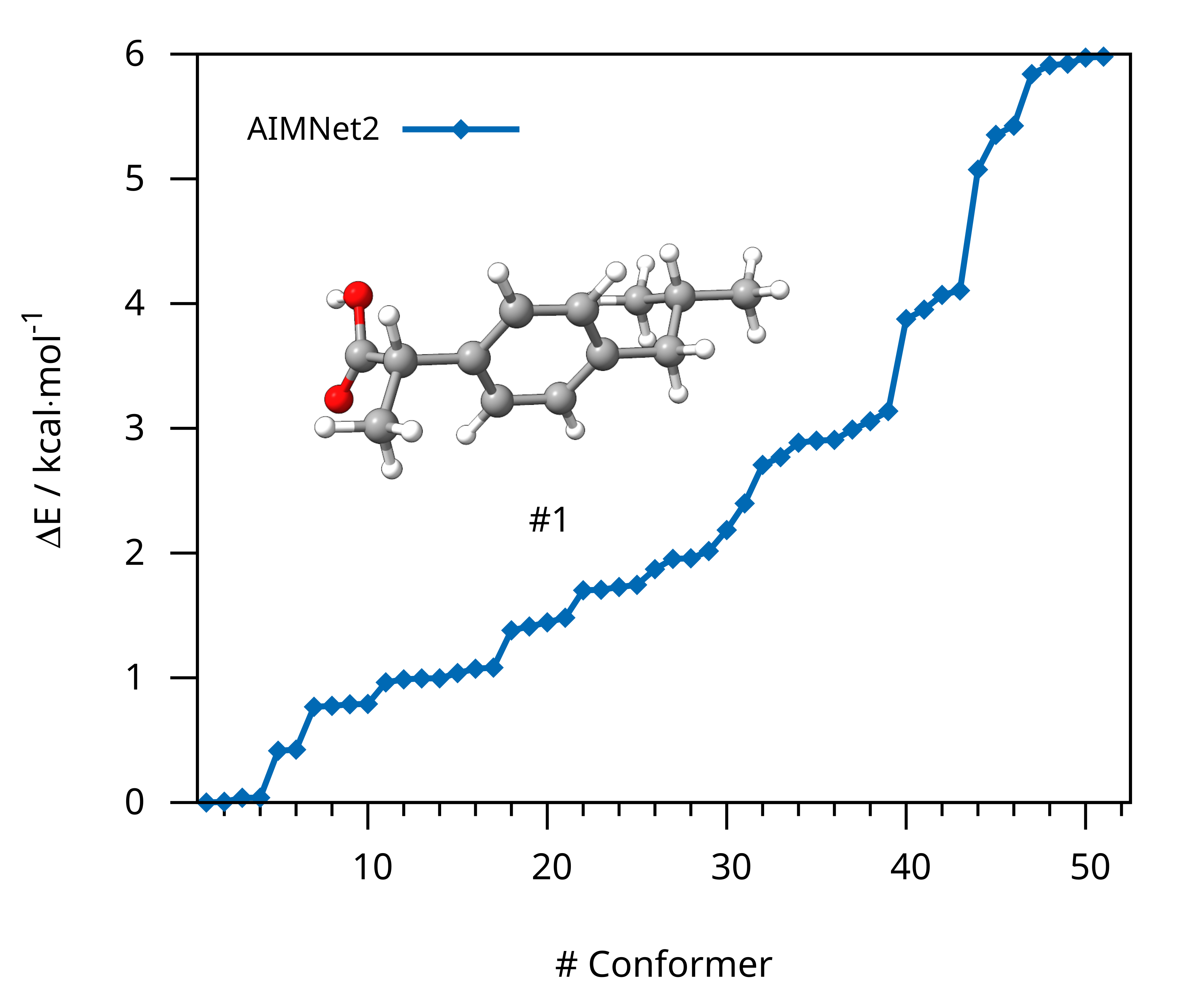
Figure: Conformer ensemble of ibuprofen generated with GOAT using AIMNet2.
Structures Example 3
Ibuprofen Input
33

 O      4.77890      0.19700      -0.13590
 C      3.44760      0.36080      -0.18720
 O      2.98080      1.45980      -0.37180
 C      2.53530     -0.82620      -0.01460
 C      2.77710     -1.46020       1.35670
 C      1.10060     -0.37560      -0.11370
 C      0.27900     -0.89600      -1.09610
 C     -1.03690     -0.48270      -1.18710
 C     -1.53140      0.45070      -0.29540
 C     -2.96590      0.90160      -0.39490
 C     -3.84720     -0.00780       0.46370
 C     -5.28200      0.52340       0.46260
 C     -3.82800     -1.42600      -0.11010
 C     -0.71030      0.97010       0.68790
 C      0.60460      0.55380       0.78130
 H      5.36430      0.95870      -0.24670
 H      2.74070     -1.55890      -0.79500
 H      2.57160     -0.72740       2.13710
 H      2.11720     -2.31870       1.48160
 H      3.81480     -1.78610       1.42840
 H      0.66540     -1.62530      -1.79280
 H     -1.67860     -0.88870      -1.95510
 H     -3.04930      1.92880      -0.03990
 H     -3.29230      0.84860      -1.43350
 H     -3.46650     -0.02390       1.48490
 H     -5.66270      0.53950      -0.55860
 H     -5.90980     -0.12450       1.07430
 H     -5.29560      1.53380       0.87140
 H     -4.20870     -1.41000      -1.13130
 H     -2.80580     -1.80450      -0.10930
 H     -4.45580     -2.07400       0.50160
 H     -1.09670      1.69900       1.38480
 H      1.24620      0.95960       1.54940
Lowest Conformer (AIMNet2)
33

O 1.89452635 2.74670433 1.65572355
C 2.46303606 1.53295140 1.81204838
O 2.81273687 1.12664895 2.88780233
C 2.56653560 0.78194831 0.50376922
C 3.67292032 -0.2677785 0.58211167
C 1.21043688 0.17850005 0.18521759
C 0.58967299 0.43999279 -1.0301631
C -0.6381833 -0.1240209 -1.3336595
C -1.2811642 -0.9653700 -0.4309326
C -2.6219811 -1.5635546 -0.7724310
C -3.7803819 -0.5563511 -0.7566304
C -5.0633632 -1.2101279 -1.2514248
C -3.9762248 0.04151965 0.63159179
C -0.6572722 -1.2227643 0.78438489
C 0.57074353 -0.6587236 1.09158276
H 1.84341759 3.13327885 2.53789267
H 2.80120095 1.50308672 -0.2766971
H 4.63561284 0.19127026 0.79559752
H 3.45485252 -0.9812724 1.37145269
H 3.73685105 -0.8010212 -0.3632347
H 1.07240053 1.09458246 -1.7441201
H -1.1056964 0.08912162 -2.2866663
H -2.5624071 -2.0075727 -1.7680116
H -2.8439965 -2.3743134 -0.0758410
H -3.5241062 0.25577994 -1.4393043
H -5.3598696 -2.0216935 -0.5853775
H -5.8800866 -0.4903223 -1.2828498
H -4.9362753 -1.6233665 -2.2511528
H -4.2296101 -0.7416544 1.34806325
H -3.0700625 0.53470069 0.97775697
H -4.7862335 0.77030765 0.63151268
H -1.1397547 -1.8767264 1.50038281
H 1.03232592 -0.8650591 2.04830637
Example 4: NEB-TS with UMA
In this example, we will run a NEB-TS transition state search of the sigmatropic shift of 5-(trimethylsilyl)-2-methyl-1,3-cyclopentadiene.
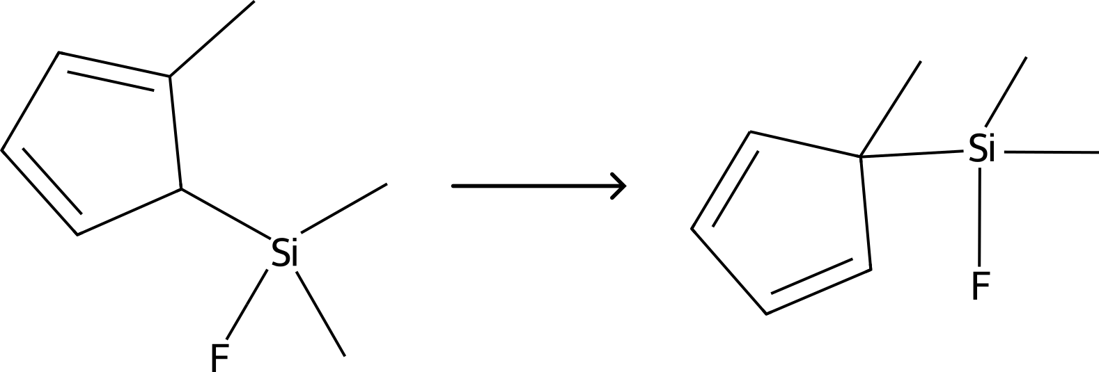
Figure: Sigmatropic shift of 5-(trimethylsilyl)-2-methyl-1,3-cyclopentadiene.
Similar to AIMNet2, we use the server/client setup. Therefore, we first start the server via oet_server:
oet_server uma
Note
Using the UMA models requires you to be logged in with your HuggingFace account (huggingface-cli login) and to have access to the UMA repository.
Then, we can provide the path to the umaclient.sh script in the ORCA input:
!ExtOpt NEB-TS PAL8

%method
  ProgExt "/full/path/to/umaclient.sh"
end

%NEB
  NEB_END_XYZFILE "products.xyz"
  PreOpt true
  NImages 15
END

*XYZFILE 0 1 reactants.xyz
Note
Once the server is initialized with uma, it can handle different models/parameterizations. If not already present, the selected model will be installed. Depending on your download speed, this might take a few minutes.
We can now run the ORCA input file as usual via orca basename.inp > basename.out and if everything is set up properly, ORCA will call fairchem via the wrapper script to calculate energies and gradients and reformat them to be readable by ORCA. The ORCA output will look the same as if the chosen task was done with any method native to ORCA.
After the successful NEB-TS run, the generated minimum energy pathway is stored as basename_MEP_trj.xyz and can be visualized using one of various
graphical user interfaces and the relative energies can be plotted.
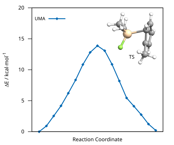
Figure: NEB-TS minimum energy path and TS guess computed with UMA.
Structures Example 4
Reactants
23

C           -4.61104849954373        3.18823292152475       -0.20905746507776
C           -4.17180337875678        1.93749036920139        0.02949708966923
H           -0.89770776274657        5.24823035215702        1.60091504658217
C           -3.43166084711657        4.08920288705507       -0.36851853894810
C           -2.73406540524902        1.91468693314661       -0.00834648022740
H           -4.78384342693541        1.07062903309282        0.20606897837631
C           -2.28086123037477        3.14997838257624       -0.27428642205396
H           -2.14144920376547        1.02885584393785        0.13908107847877
Si          -3.33332222092925        5.37907495289466        1.05277770096436
C           -6.02097164061157        3.66317446803335       -0.27653426232915
H           -1.25885613496678        3.45990279108919       -0.39136845245007
H           -6.12104057192362        4.48363161298959       -0.98515577017189
H           -6.35176539913037        4.01532788571936        0.70180780527581
H           -6.68040967896903        2.85226254487986       -0.57914614531044
C           -4.59856418636902        6.78018321279534        0.85045329008624
F           -3.72652768685745        4.59638629973297        2.42356736138995
C           -1.57323319430198        6.04135354820534        1.29568183762139
H           -5.61717266687775        6.41367954591729        0.93225375074929
H           -4.45932873451201        7.52935407107000        1.62422459431827
H           -4.50305527286240        7.27890449031607       -0.10935364145480
H           -1.17624027092519        6.48608325952275        0.38892789807178
H           -1.55496107155660        6.80247969646478        2.06985275156072
H           -3.44875735451884        4.63379919897783       -1.31332880312171
Product
23

C           -4.69990994976011        3.20924065322322        0.09962483278590
C           -3.99840024883976        1.90401213276398        0.20416516977898
H           -2.37158991505561        3.22667232627870        2.41126692401130
C           -3.72694648280184        4.03533797051083       -0.66137023857848
C           -2.76428353419624        2.01160573997675       -0.32104212597326
H           -4.44231122338321        1.04008250088565        0.66262339362888
C           -2.59618051337500        3.33421765463529       -0.85922199874793
H           -2.01172244318102        1.24335106555387       -0.36018756997101
Si          -4.71935970533593        3.91779868936117        1.89798478659303
C           -6.10977295078427        3.14892887568830       -0.47700242310846
H           -1.70115130949351        3.67861323625581       -1.34731175401222
H           -6.53144611076232        4.14723750560114       -0.56923985079405
H           -6.75797855532321        2.55181698634220        0.16023505831658
H           -6.08132877026183        2.69487084388844       -1.46588884873030
C           -5.75674328208435        5.50195935857526        2.01424211607064
F           -5.52419505568003        2.80526301087179        2.78290540700344
C           -2.99119773357252        4.08564756120852        2.64875310499782
H           -6.80434705475406        5.29926403052655        1.81229976499256
H           -5.69377703675228        5.92291704242447        3.01272638872414
H           -5.42249276211225        6.26148436294309        1.31518712332358
H           -2.48112101016319        4.96988971061287        2.28209513286334
H           -3.05482787696738        4.16178477761192        3.72960656803603
H           -3.93181814405995        5.04388417875953       -0.97098171851138
Example 5: NEB-TS with g-xTB
In this example, we will run a NEB-TS transition state search of a hydride transfer reaction with g-xTB. The g-xTB binary can be obtained from Grimme lab and the wrapper script for running g-xTB in ORCA can be obtained from our ORCA-External-Tools GitHub repository. After the g-xTB binary is downloaded the parameter files from the repository have to be added to the home directory ~/ or specified in the ORCA input. Then the NEB calculation can be started via:
Warning
The g-xTB binary is a preliminary version that currently works only on Linux-based systems. Gradients are computed numerically. Therefore, the gradient calculations take a significant time, slowing down applications that compute gradients often like GOAT.
!ExtOpt NEB-TS FREQ NUMFREQ

%method
  ProgExt "/full/path/to/oet_gxtb"
end

%NEB
  NEB_END_XYZFILE "product.xyz"
END

*XYZFILE -1 1 reactant.xyz
As before, we can now run the ORCA input file as usual via orca basename.inp > basename.out and if everything is set up properly, ORCA will call g-xTB via the wrapper script to calculate energies and gradients and reformat them to be readable by ORCA. The ORCA output will look the same as if the chosen task was done with any method native to ORCA.
After the successful NEB-TS run, the generated minimum energy pathway is stored as basename_MEP_trj.xyz and can be visualized using one of various
graphical user interfaces:
Figure: NEB-TS minimum energy path with g-xTB.
Structures Example 5
Reactant
26

C         1.075372    0.593011    1.070561
C         2.400034    0.861951    0.344585
C         3.262960   -0.389376    0.095361
C         2.336297   -1.332404   -0.764449
C         0.902274   -1.426701   -0.341781
C         0.305638   -0.558970    0.472502
H         0.306315   -2.251280   -0.737622
C        -1.169823   -0.650551    0.790263
C        -2.025300   -0.056133   -0.333804
H        -1.393212   -0.123082    1.724642
H        -1.481857   -1.685477    0.934655
C        -3.526989   -0.190041   -0.057081
O        -4.031191   -1.151571    0.455482
O        -4.239688    0.858934   -0.477431
N        -1.729463    1.338834   -0.683787
H        -1.848609   -0.653247   -1.233619
O         4.459293   -0.236543   -0.413208
O         2.673236    1.996721    0.023440
H        -3.565539    1.485831   -0.830121
H        -1.455642    1.864108    0.140364
H        -0.944726    1.390619   -1.322680
H         2.408545   -0.963628   -1.795585
H         2.809257   -2.318530   -0.767668
H         0.496836    1.522242    1.055312
H         1.287847    0.379685    2.125786
H         3.231045   -0.864118    1.129829
Product
26

C         1.051874   -0.848598   -0.267729
C         2.598645   -0.805502   -0.564168
C         3.120016    0.372226    0.281378
C         2.418841    1.718563    0.046113
C         0.956912    1.612933   -0.274430
C         0.312284    0.455326   -0.403339
H         0.408475    2.545929   -0.392802
C        -1.163475    0.438406   -0.717988
C        -2.048393   -0.050235    0.440681
H        -1.352218   -0.207194   -1.585352
H        -1.502168    1.441778   -0.979784
C        -3.516320    0.254910    0.114235
O        -3.961146    1.368848    0.039359
O        -4.251921   -0.836174   -0.097995
N        -1.910568   -1.492712    0.686599
H        -1.797263    0.538460    1.326851
O         4.037141    0.320454    1.067845
O         3.173485   -1.974283   -0.439530
H        -3.620184   -1.580034    0.065611
H        -1.074783   -1.863714    0.250474
H        -1.841358   -1.697033    1.675761
H         2.584233    2.337228    0.934522
H         2.945797    2.222498   -0.774052
H         0.961210   -1.262690    0.744536
H         0.651768   -1.603074   -0.954904
H         2.647697   -0.342098   -1.603003
Writing your own scripts
If you want to use a method with ORCA that is not currently available, you can either open an issue on GitHub or implement it yourself. To simplify this process, the, the ORCA-External-Tools GitHub repository provides a modular framework. Only the interface between ORCA and your chosen method needs to be implemented.
To add a new method:
Create a new calculator class that inherits from the
BasicSettingsclass.Override the
calcroutine to define the calculation logic.Define the
mainroutine following the examples provided in existing calculators.Add your new calculator to the list of available calculators in
base_calc.py.
These calculators are usually able to run on the provided server functionality without further modifications.