Electrostatic Potentials (ESP)¶

The Molecular Electrostatic Potentials (ESP, MESP, or MEP) can be described as the potential energy of a positive probe charge interacting with the charge cloud of a molecule. Even though it does not describe any polarization effects, the ESP is a useful tool to identify electrophilic sites within a molecule and thus give hints to its reactivity.

Starting with ORCA 6.1, the ESP can be generated via the orca_plot utility for any state density generated in an electronic structure calculation with ORCA.

Example: ESP of Sulfanilic Acid¶

In this example, we will compute the ESP of Sulfanilic Acid, an key reagent for the synthesis of Lunges reagent and diazo dyes.

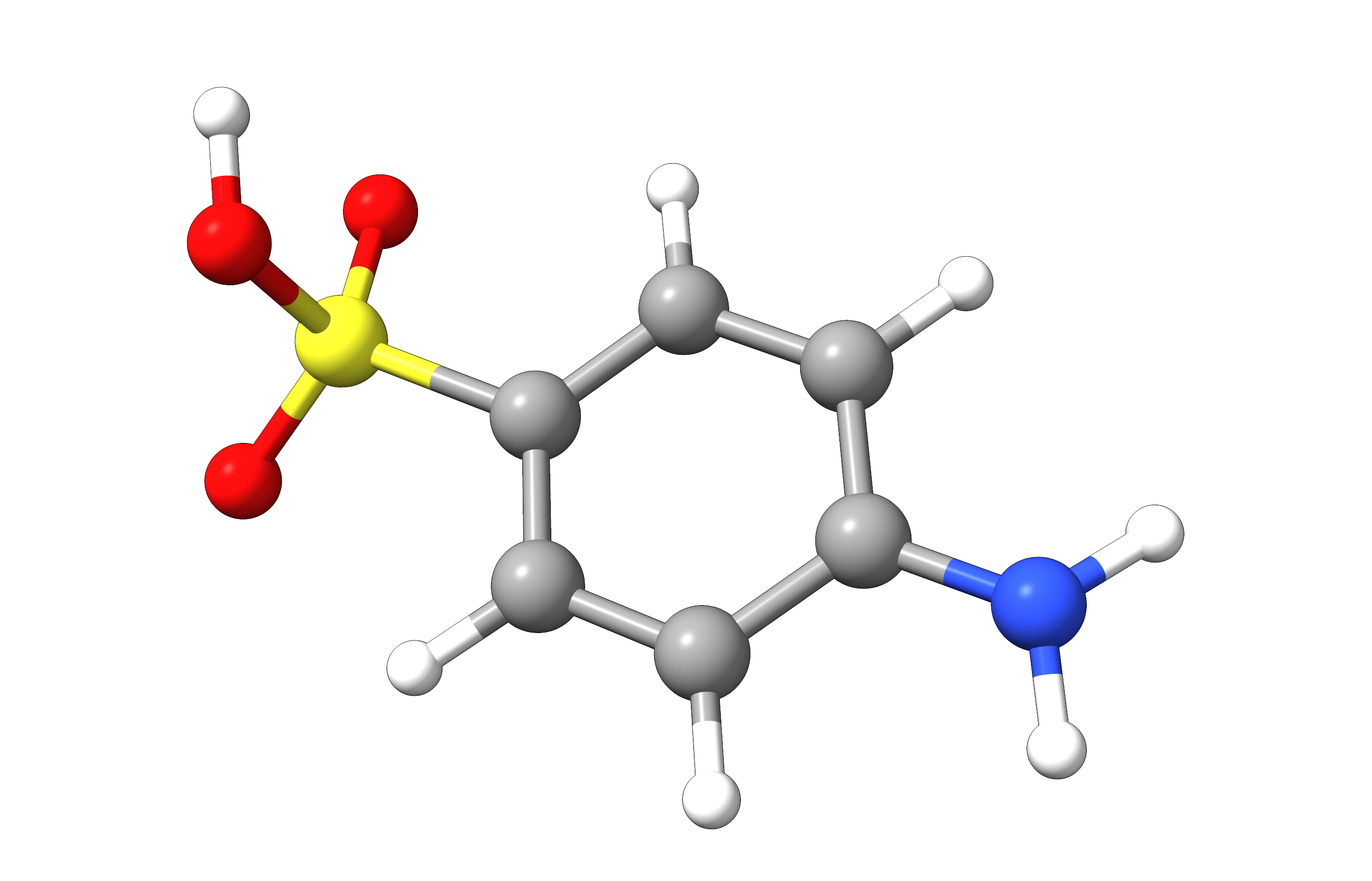
../_images/struc-sulfanilic-acid.png — Figure: Molecular structure of sulfanilic acid.¶

In principle we can use any density generating electronic structure method within ORCA to compute the ESP on. In this example we chose the r²SCAN0/def2-SVP level of theory. First, we perform a SCF calculation at this level on a previously optimized geometry of sulfanilic acid.

! r2SCAN0 def2-SVP

*xyzfile 0 1 sulfanilicacid.xyz

This calculation will store the required electronic density file in its orca.densities container. To visualize the ESP, we have to generate two .cube files, one of the electronic density and one of the electrostatic potential.

Both can be generated via orca_plot. The graphical interface of orca_plot is invoked via orca_plot orca.gbw -i.

[...]

Current-settings:

PlotType id    ... 2
PlotType       ... DENSITY-PLOT
ElDens File    ... orca.scfp
Output file    ... MyElDens
Format         ... Grid3d/Cube
Resolution     ... 100 100 100
Boundaries     ...   -15.128411    12.322825 (x direction)
                     -11.045609    11.042514 (y direction)
                     -10.422121     8.237903 (z direction)

       1 - Enter type of plot
       2 - Enter no of orbital to plot
       3 - Enter operator of orbital (0=alpha,1=beta)
       4 - Enter number of grid intervals
       5 - Select output file format
       6 - Plot CIS/TD-DFT difference densities
       7 - Plot CIS/TD-DFT transition densities
       8 - Set AO(=1) vs MO(=0) to plot
       9 - List all available densities
      10 - Perform Density Algebraic Operations

      11 - Generate the plot
      12 - exit this program
Enter a number:

Tip

In this example, we increased the number of grid points to 100x100x100 via the option 4 - Enter number of grid intervals. This is typically sufficient for publication purposes. Note that larger grids also result in larger files and increased generation time.

To generate the cube file containing the electron density, we choose 1 - Enter type of plot\(\rightarrow\)2 - (scf) electron density

-----------------------------------------------------------------------
Reading Over   2 Saved Densities                                    ...
-----------------------------------------------------------------------
-----------------------------------------------------------------------
Plot-Type is presently: 2
-----------------------------------------------------------------------
Searching for Ground State Electron or Spin Densities:              ...
-----------------------------------------------------------------------
     1 -   molecular orbitals                          
     2 -   (scf) electron density                              ......  (scfp                     )  => AVAILABLE
[...]

and confirm to use the the default density orca.scfp from the density container.

The default name of the density would be: orca.scfp
Is this the one you want (y/n)? y

We can now set the output format to .cube via 5 - Select output file format\(\rightarrow\)7 - 3D Gaussian cube and use 11 - Generate the plot to generate the orca.eldens.cube file. Next, we generate the electrostatic potential via 1 - Enter type of plot\(\rightarrow\)43 - Electrostatic Potential.

[...]
    41 -   ROCIS QDPT unrelaxed transition AO density          ......  (Tdens-ROCISQDSOC         )  - NOT AVAILABLE
    42 -   LFT QDPT unrelaxed transition AO density            ......  (Tdens-LFTQDSOC           )  - NOT AVAILABLE
-----------------------------------------------------------------------
    43 -   Electrostatic Potential 

We are again asked, which density should be used and choose the standard electron density orca.scfp.

---------------------
List of density names
---------------------

Index:                                                   Name of Density
------------------------------------------------------------------------
    0:                                                         orca.scfp
    1:                                                       orca.P0.tmp


Enter Name for an STATE Density: orca.scfp

Finally we can start the calculation of the electrostativ potential via 11 - Generate the plot. Note that this can take some time depending on the number of grid points chosen. The electrostatic potential data will then be stored in the orca.scfp.esp.cube file.

In principle, we should now have the following files ready to plot our ESP with ChimeraX:

sulfanilicacid.xyz that contains the cartesian coordinates of the input molecule
orca.eldens.cube that contains the electron density
orca.scfp.esp.cube that contains the electrostatic potential

We now load the three files in that order into ChimeraX and enter the following command into its command line (sometimes pressing enter twice is required to apply the coloring):

volume #3 hide; volume #2 level 0.001; color electrostatic #2 map #3 range full palette ^rainbow key true transparency 60

Basically, this will hide the raw esp file, set the isosurface value of the electron density to 0.001 a.u., and colorize the density surface by the electrostatic potential data. ChimeraX offers a variety of additional visualization options. The plot can now be saved as a .PNG file and we can now easily identify regions of strong attractive interaction with the positive point charge colored in red.

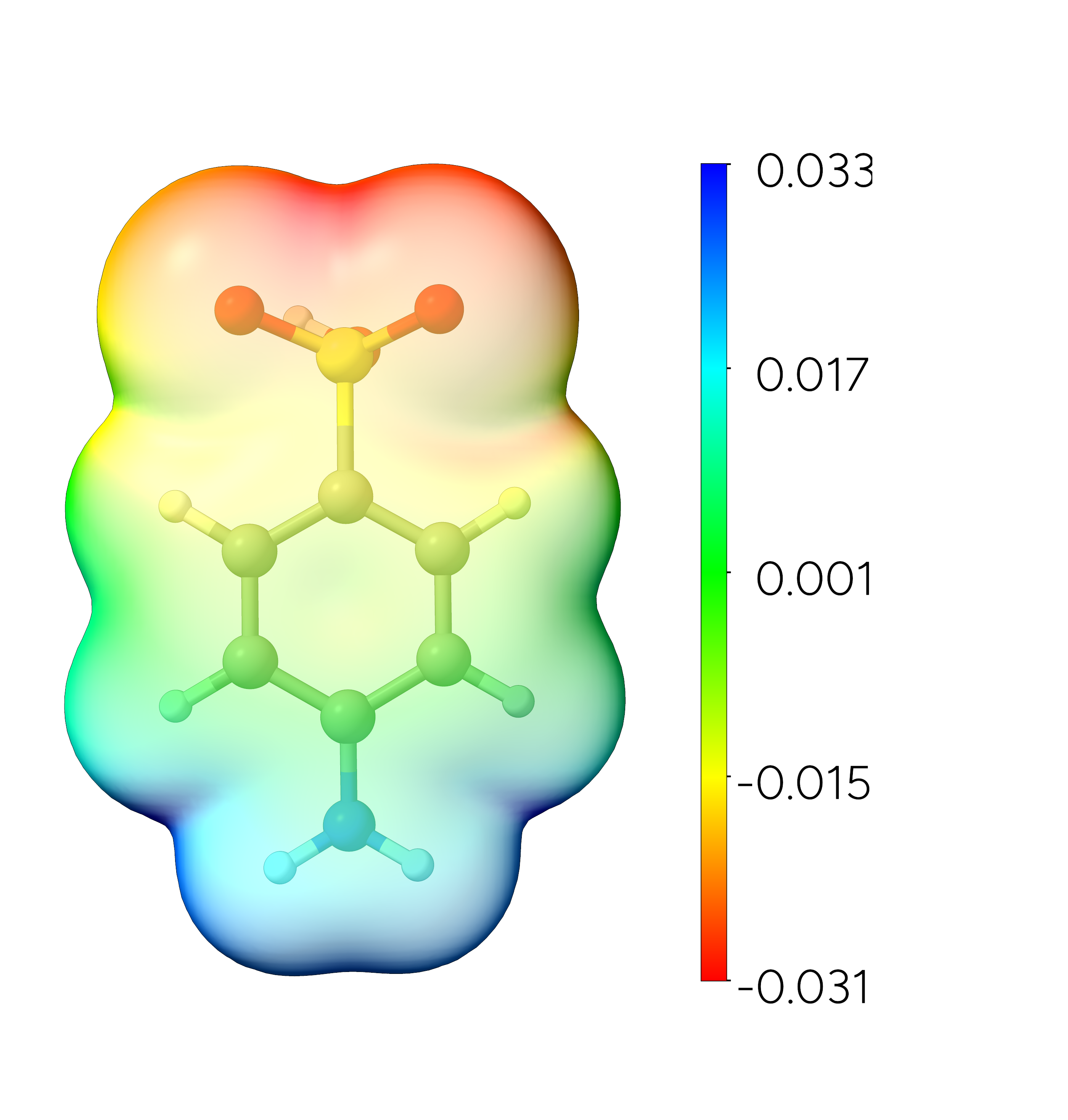
../_images/esp-sulfanilic-acid.png — Figure: Molecular electrostatic potential mapped to the electron density of sulfanilic acid. Isosurface value = 0.001 a.u.¶

Electrostatic Potentials (ESP)¶

Example: ESP of Sulfanilic Acid¶

Structures¶