Nuclear Magnetic Resonance (NMR)
General Use
NMR spectroscopy is a powerful tool to analyze the structural features of any molecule. In ORCA, NMR spectroscopic properties like shielding tensors and shifts, J coupling constants, and NMR spin-rotation constants can be calculated. These properties can be calculated by a wide range of different methods and we generally recommend to check recent benchmark studies like those by Kaupp and co-workers to [Kaupp2021a][Kaupp2021b] find a suitable method.
Important
The pcSseg-2 and pcSseg-1 basis sets used in some of the following tutorials are only available up to Kr. If heavier elements are present for which you don't want to compute the NMR properties anyway, you may add another available basis set like def2-TZVP with the respective ECP to these atoms instead. For more information check the ORCA manual.
NMR Shielding Tensors
A basic NMR shielding tensor calculation can be requested by the NMR input keyword.
!BP86 DEF2-TZVP NMR

*XYZFILE 0 1 structure.xyz
This input will compute the shielding tensors for all nuclei present in the given molecule.
J Coupling Constants
J coupling constants can be requested via the SSALL keyword in the %EPRNMR block:
!BP86 DEF2-TZVP NMR

* XYZFILE 0 1 structure.xyz

%EPRNMR
     NUCLEI = ALL H {SHIFT, SSALL}
END
Important
The %EPRNMR block must be placed after the coordinates specification!
Hint
The SHIFT keyword in the example above will limit the computed shieldings to the H-atoms.
Spin-Rotation Constants
Spin-rotation constants can be requested by the SROT keyword.
!BP86 DEF2-TZVP MASS2016

*XYZ 0 1
  C          -1.98519000000000      1.12204043805165      0.00000000000000
  O          -1.98519000000000     -0.00136043805165      0.00000000000000 M=16.999131
*

%EPRNMR
  NUCLEI = ALL O {SROT, IST=17}
END
Note
We have to define the masses of the individually requested nuclei via the coordinates input! The MASS2016 keyword will only use the atomic masses for the most abundant isotope that were
redetermined in 2016. The IST keyword defines the magnetogyric ratio that will be used via the chosen isotope, in this case 17O.
Warning
The ORCA implementation follows that described in [Helgaker1996]. Therefore, the sign convention of the rotation constant components may differ when compared to different sources.
Example 1: 13C-NMR Chemical Shifts of Propionic Acid
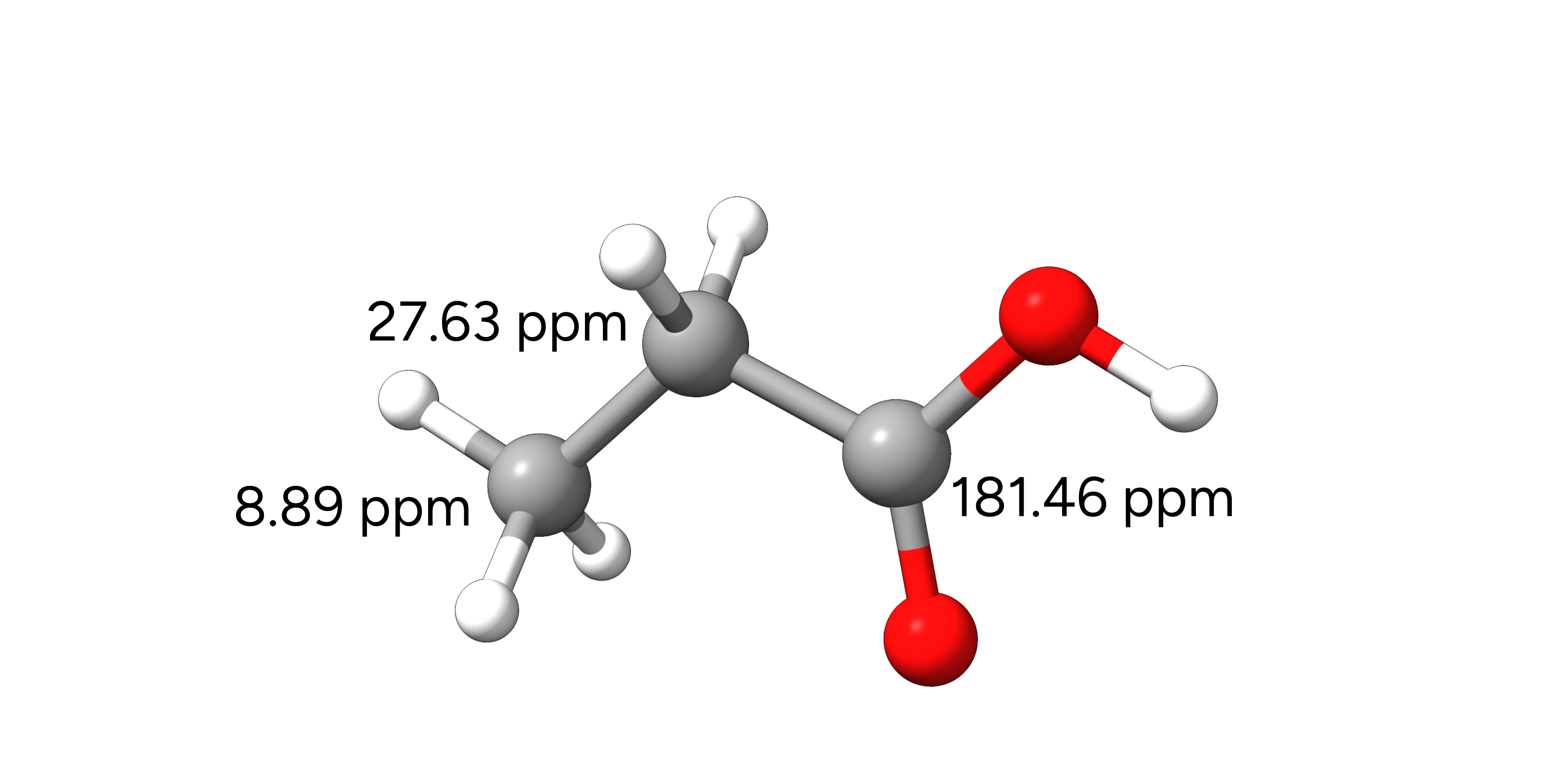
In this example, we will compute the isotropic shieldings of the 13C nuclei of propionic acid in CHCl3 solution. Experimental data for this molecule can be found in the SDBS database.

Figure: Molecular structure of propionic acid and the experimental 13C NMR chemical shifts.
These will be used to compute the chemical shifts of the respective nuclei with reference to TMS according to:
Important
For very large shielding tensors, e.g. of very heavy nuclei such as Pb, the denominator (\(1 - \sigma_{ref.})\) cannot be neglected anymore.
As we use TMS as reference, we will first compute the isotropic shieldings for the TMS molecule with the TPSS meta-GGA functional and Jensen's pcSseg-1 basis set. TPSS typically yields reasonably good NMR properties for most nuclei. Note, that for more accurate results, at least triple-Zeta basis sets like pcSseg-2 or def2-TZVP should be used.
Important
For meta-GGA functionals like TPSS, a gauge-invariant option for the treatment of the kinetic energy density should be used! The current density-dependent, gauge-invariant version of the approach by Dobson is recommended and can be invoked by TAU DOBSON in the %EPRNMR block.
!TPSS PCSSEG-1 AUTOAUX NMR CPCM(CHCl3)

%EPRNMR
   TAU DOBSON
END

*XYZFILE 0 1 tms.xyz
Hint
Instead of calculating a reference molecule you can use an internal standard. In this case, you just apply a constant shift to the calculated peaks, so that one of them is equal to a known value. For example, one could use the value of an assigned methyl or an aromatic H or C and benefit from possible error cancellations. This also makes more sense if the reference is too different from the target molecule or complicated to simulate, like phosphoric acid in water for 31P-NMR.
After the successful SCF calculation, ORCA will initiate the property calculation summarizing the requested properties:
Tau option for meta-GGA DFT with GIAOs    ... Dobson

[...]

------------------------------------------------------------------------------
                              ORCA PROPERTY CALCULATIONS
------------------------------------------------------------------------------

GBWName                                 ... orca.gbw
Number of atoms                         ...     17
Number of basis functions               ...    152
Max core memory                         ...   4096 MB

[...]

NMR properties:
Chemical shifts                         ... YES (  17 nuclei)
Spin-rotation constants                 ...  NO (   0 nuclei)                   Spin-spin couplings                     ...  NO (   0 nuclei,    0 pairs)

Choice of magnetic origin               ... GIAO
Position of magnetic origin             ...     0.000000     0.000000     0.000000
Note
The default algorithm uses Gauge-Independent Atomic Orbitals (GIAOs, [Ditchfield1973] and [Pulay1990]). This is quite important in NMR calculations and we do not recommended turning this off unless you really know what you are doing.
The calculated NMR shieldings are now printed after:
-------------------
CHEMICAL SHIELDINGS (ppm)
-------------------
with more detailed information on the computed components for each individual nucleus.
 --------------
 Nucleus   1C :
 --------------

Diamagnetic contribution to the shielding tensor (ppm) :
           250.664          0.000         0.011
             0.000        250.666         0.000
             0.002          0.000       261.510

Paramagnetic contribution to the shielding tensor (ppm):
           -68.478         -0.000         0.069
            -0.000        -68.472        -0.000
            -0.028         -0.000       -72.311

Total shielding tensor (ppm):
           182.186         -0.000         0.080
            -0.000        182.194        -0.000
            -0.026         -0.000       189.198


 Diagonalized sT*s matrix:

 sDSO           250.665          250.666          261.510  iso=     254.280
 sPSO           -68.478          -68.472          -72.311  iso=     -69.754
        ---------------  ---------------  ---------------
 Total          182.186          182.194          189.198  iso=     184.526

 Orientation:
  X          -0.9998887   -0.0144421    0.0037505
  Y          -0.0144423    0.9998957   -0.0000096
  Z           0.0037499    0.0000637    0.9999930
The desired isotropic shieldings are further summarized:
--------------------------------
CHEMICAL SHIELDING SUMMARY (ppm)
--------------------------------


  Nucleus  Element    Isotropic     Anisotropy
  -------  -------  ------------   ------------
      0       Si         353.498          0.067
      1       C          184.526          7.008
      2       C          184.513          7.061
      3       C          184.549          6.996
      4       C          184.549          6.996
[...]
Note
Chemically equivalent nuclei might have slight different shieldings, due to geometric asymmetries. In that case, the best thing to do is to simply average them.
After we got our reference shieldings for TMS, we can now calculate the respective 13C shieldings for propionic acid:
!TPSS PCSSEG-1 AUTOAUX NMR CPCM(CHCl3)

*XYZFILE 0 1 propionic_acid.xyz

%EPRNMR
   NUCLEI = ALL C {SHIFT}
   TAU DOBSON
END
--------------------------------
CHEMICAL SHIELDING SUMMARY (ppm)
--------------------------------


  Nucleus  Element    Isotropic     Anisotropy
  -------  -------  ------------   ------------
      0       C          172.914         13.514
      1       C          155.500         33.193
      5       C            6.568       -132.026
We can now calculate the respective chemical shifts and see that they are in reasonable agreement with the experimental data.
Method |
\(\delta_1\) |
\(\delta_2\) |
\(\delta_3\) |
|---|---|---|---|
TPSS/pcSseg-1 |
11.6 |
29.0 |
178.0 |
TPSS/pcSseg-2 |
11.6 |
30.1 |
184.4 |
TPSSh/pcSseg-2 |
11.8 |
30.5 |
185.9 |
Exp. |
8.9 |
27.6 |
181.5 |
Note
Have in mind that the refence should always use the same level of theory as the target molecule, including any solvation effects or approximations such as the RI.
Important
Always have in mind that NMR shifts are quite sensitive to the conformer you choose. For flexible molecules, a conformer search with GOAT and subsequent Boltzmann weighting of the NMR properties for the conformer ensemble should be considered!
Example 2: J(H-H) Coupling Constants of Toluene and Plot with ChimeraX
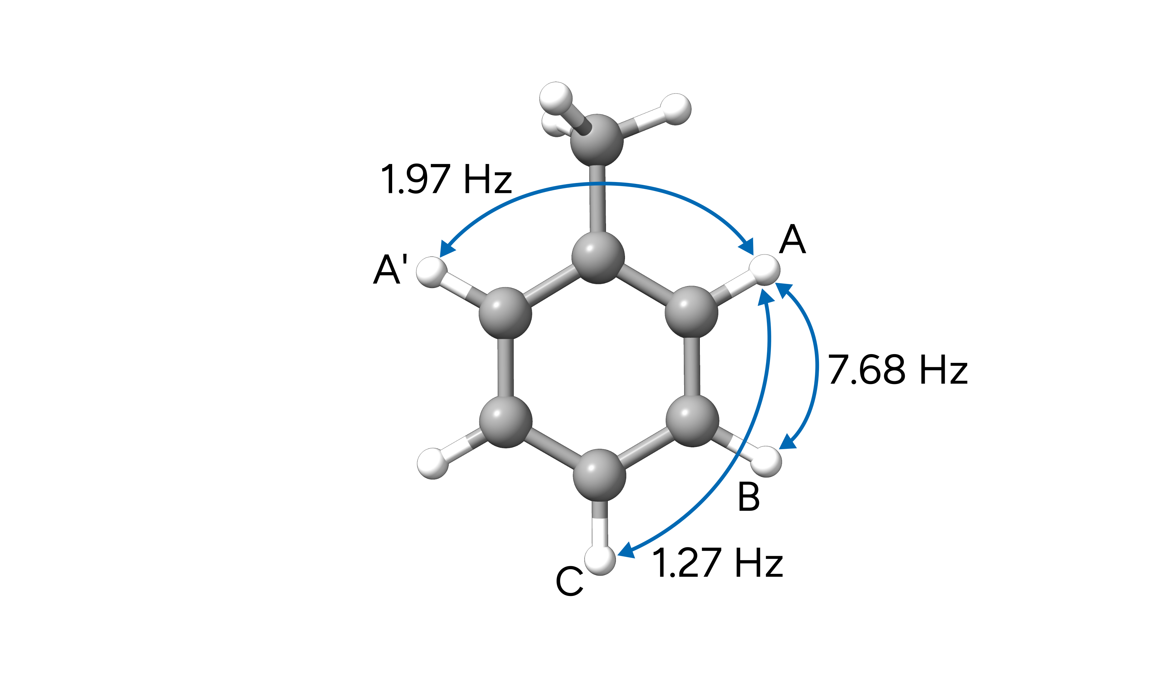
In this example, we calculate the J(H-H) couplings of toluene in chloroform for which experimental data are again extracted from the SDBS database. Here we highlight some of the J couplings between hydrogen atoms of the aromatic ring, as labeled in the database:

Figure: Selected experimental J(H-H) coupling constants of toluene.
We use a similar input as used in the previous example and add the SSALL keyword.
!TPSS PCSSEG-1 AUTOAUX NMR CPCM(CHCl3)

*XYZFILE 0 1 toluene.xyz

%EPRNMR
   NUCLEI = ALL H {SHIFT, SSALL}
   TAU DOBSON
END
The output will now show the details on the computed coupling constants:
-----------------------------------------------------------------------
                     NMR SPIN-SPIN COUPLING CONSTANTS
                     ================================

    Number of nuclear pairs to calculate something:       22
                                                        ----
    Number of nuclear pairs to calculate DSO   terms:     22
    Number of nuclear pairs to calculate PSO   terms:     22
    Number of nuclear pairs to calculate FC    terms:     22
    Number of nuclear pairs to calculate SD    terms:     22
    Number of nuclear pairs to calculate SD/FC terms:     22
-----------------------------------------------------------------------

Performing DSO num. integration        ... done (   0.1 sec)

Processing PSO nuclear pairs   ... done (   0.0 sec)
Processing SD/FC nuclear pairs ... done (   0.0 sec)

-----------------------------------------------------------
 NUCLEUS A = H    0 NUCLEUS B = H    3
 (  1H  gnA =  5.586   1H  gnB =  5.586) r(AB) =     2.4644
-----------------------------------------------------------

Diamagnetic contribution to J (Hz):
        3.9268         3.7449       -0.0013
       -3.8794        -3.6900        0.0009
        0.0006         0.0003       -1.2663
Paramagnetic contribution to J (Hz):
       -2.2397        -3.1792        0.0010
        3.2992         2.1041       -0.0007
       -0.0006        -0.0002        0.5562
Fermi-contact contribution to J (Hz):
        6.2432         0.0000        0.0000
        0.0000         6.2432        0.0000
        0.0000         0.0000        6.2432
Spin-dipolar contribution to J (Hz):
        0.1973         0.2594       -0.0001
       -0.2592         0.1564       -0.0000
        0.0000        -0.0001       -0.0915
Spin-dipolar/Fermi contact cross term contribution to J (Hz):
       -0.2582        -0.0105        0.0000
       -0.0105         0.0912        0.0000
        0.0000         0.0000        0.1675

Total spin-spin coupling tensor J (Hz):
        7.8694         0.8146       -0.0004
       -0.8498         4.9049        0.0003
        0.0000         0.0002        5.6091

 Diagonalized JT*J matrix:

 J[0,3](DSO)           -3.656           -1.266            3.893  iso=     -0.343
 J[0,3](PSO)            2.082            0.556           -2.218  iso=      0.140
 J[0,3](FC)             6.243            6.243            6.243  iso=      6.243
 J[0,3](SD)             0.157           -0.091            0.197  iso=      0.087
 J[0,3](SD/FC)          0.091            0.167           -0.258  iso=      0.000
              ---------------  ---------------  ---------------  ---------------
 J[0,3](Total)          4.917            5.609            7.857  iso=      6.128

[...]
With a final summary in the end:
-----------------------------------------------------------------------------
                SUMMARY OF ISOTROPIC COUPLING CONSTANTS J (Hz)
-----------------------------------------------------------------------------
                  0 H        3 H        7 H        9 H       11 H       12 H
      0 H        0.000      6.128      0.353      1.152      5.984     -0.075
      3 H        6.128      0.000      1.545      0.309      0.939      0.261
      7 H        0.353      1.545      0.000      6.286      0.921     -0.230
      9 H        1.152      0.309      6.286      0.000      5.829      0.000
     11 H        5.984      0.939      0.921      5.829      0.000      0.000
     12 H       -0.075      0.261     -0.230      0.000      0.000      0.000
     13 H        0.000     -1.286     -0.922      0.145      0.000    -13.479
     14 H        0.000     -1.281     -0.914      0.143      0.000    -13.464
                 13 H       14 H
      0 H        0.000      0.000
      3 H       -1.286     -1.281
      7 H       -0.922     -0.914
      9 H        0.145      0.143
     11 H        0.000      0.000
     12 H      -13.479    -13.464
     13 H        0.000    -17.265
     14 H      -17.265      0.000
Important
The values are printed in Hz, so in order to convert them to ppm one has to take into account the equipment's frequency. In our case, the database says it was measured in 300 MHz NMR, so that the coupling in ppm would be:
Again, we can compare our computed data to the experiment:
Coupling |
Calculated (Hz) |
Experiment (Hz) |
|---|---|---|
TPSS/pcSseg-1 |
||
A (H3) - A' (H7) |
1.15 |
1.97 |
A (H7) - B (H9) |
6.29 |
7.68 |
A (H7) - C (H11) |
0.92 |
1.27 |
TPSS/pcSseg-2 |
||
A (H3) - A' (H7) |
2.70 |
1.97 |
A (H7) - B (H9) |
7.22 |
7.68 |
A (H7) - C (H11) |
1.82 |
1.27 |
TPSSh/pcSseg-2 |
||
A (H3) - A' (H7) |
2.49 |
1.97 |
A (H7) - B (H9) |
7.42 |
7.68 |
A (H7) - C (H11) |
1.65 |
1.27 |
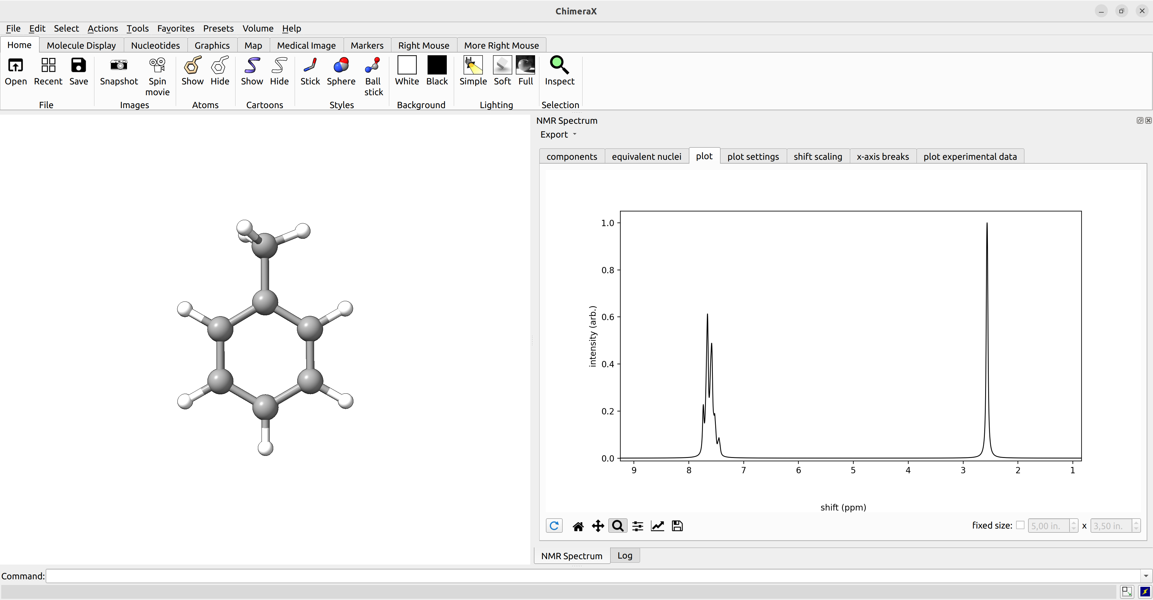
After we computed the NMR shieldings and J coupling constants, we can visualize the coupled NMR spectrum with ChimeraX (with the SEQCROW plugin).
To do so, we simply open the ORCA output file with ChimeraX, navigate to Tools→Quantum Chemistry→NMR Spectrum.
ChimeraX offers many settings, including the choice of a reference shift, the pulse frequency, and manual choice of equivalent nuclei. The spectrum can further be exported as picture or as .csv data for further processing.

Figure: Calculated NMR spectrum of toluene visualized with ChimeraX.
Example 3: NMR Chemical Shifts with Double-Hybrid DFT
In ORCA, the NMR shielding constants can also be computed using the double-hybrid functionals, that profit from adding MP2 correlation to DFT [Neese2018].
!revDSD-PBEP86-D4/2021 PCSSEG-3 AUTOAUX NMR NOFROZENCORE

*XYZFILE 0 1 opt.xyz
Important
Per default MP2 and double-hybrid DFT uses the frozen core approximation. As NMR properties are strongly influenced by the core electrons, we need to deactivate it
with the NOFROZENCORE keyword.
Note
Note, that double-hybrid functionals typically require larger basis sets like pcSseg-3 for converged results.
ORCA will compute the NMR properties at the SCF DFT level first:
-------------------
CHEMICAL SHIELDINGS (ppm)
-------------------

Method             : SCF
Type of density    : Electron Density
[...]
and the properties based on the unrelaxed and the relaxed MP2 density afterwards:
-------------------
CHEMICAL SHIELDINGS (ppm)
-------------------

Method             : MP2
Type of density    : Electron Density
Type of derivative : Magnetic Field (with GIAOs) (Direction=X)
Multiplicity       :   1
Level              : Unrelaxed density
-------------------
CHEMICAL SHIELDINGS (ppm)
-------------------

Method             : MP2
Type of density    : Electron Density
Type of derivative : Magnetic Field (with GIAOs) (Direction=X)
Multiplicity       :   1
Level              : Relaxed density
The results based on the relaxed density are the desired properties.
Warning
Double-hybrids typically give better results than lower-level DFT approaches, however, for some systems, e.g., those with small HOMO-LUMO gaps or 3d transition metal complexes, MP2-based approaches are prone to large errors and may be avoided in favor of a robust meta-GGA like B97M-V and r2SCAN or hybrid functionals like r2SCAN0, TPSSh, and ωB97X-V.
Tip
Even though no J coupling constants are available from MP2 or double-hybrid DFT, coupled spectra can be obtained from mixing theories for shieldings and couplings. For example, we can combine chemical shifts calculated at the double-hybrid DFT level with J coupling constants from a hybrid DFT calculation.
Example 4: Spin-Rotation Constants of 12C17O
In this example, we will compute the NMR spin-rotation constant of 12C17O. In the respective input, we defined the atomic mass of O to match 17O and adjusted the magnetogyric ratio for the chosen isotope.
! TPSSh PCSSEG-3 AUTOAUX MASS2016

*XYZ 0 1
  C          -1.98519000000000      1.12204043805165      0.00000000000000
  O          -1.98519000000000     -0.00136043805165      0.00000000000000 M=16.999131
*

%EPRNMR
   NUCLEI = ALL O {SROT, IST=17}
   TAU DOBSON
END
After successful calculation, the results are printed to the output.
---------------------------
NMR SPIN-ROTATION CONSTANTS
---------------------------

Analytic diamagnetic shielding integrals (local origin) (SHARK)        ... done (  0.1 sec)

 ------------------------------------------------
 Nucleus   1O  (Isotope =  17 GN =  -0.75751600):
 ------------------------------------------------

Nuclear contribution to the spin-rotation tensor (kHz) :
            -3.535          0.000         0.000
             0.000          0.000         0.000
             0.000          0.000        -3.535

Electronic contribution to the spin-rotation tensor (kHz) :
            36.353          0.000         0.000
            -0.000          0.000         0.000
             0.000          0.000        36.352

Total spin-rotation tensor (kHz):
            32.818          0.000         0.000
            -0.000          0.000         0.000
             0.000          0.000        32.817


 Diagonalized MT*M matrix:

 M(Nuc)           0.000           -3.535           -3.535  iso=      -2.356
 M(El)            0.000           36.352           36.353  iso=      24.235
        ---------------  ---------------  ---------------
 M(Tot)           0.000           32.817           32.818  iso=      21.878
here M(Tot) gives the aa, bb, and cc (or XX, YY, and ZZ) components and the isotropic NMR spin-rotation constant. The latter is further summarized in the end with some additional information like the atomic mass.
-----------------------------------
NMR SPIN-ROTATION CONSTANTS SUMMARY
-----------------------------------

  Nucleus  Isotope  Atomic Mass   g-factor   Spin-Rot. Const. (kHz)
  -------  -------  -----------  ----------  ----------------------
      1     17-O     16.9991310  -0.7575160            21.878
If we now compare the spin-rotation constant components with the experiment, we see that the absolute value is in excellent agreement with the experimental data. Note that the sign convention used in the original implementation followed in ORCA[Helgaker1996] may differ from that used in other works.
Component |
Calculated (kHz) |
Experiment (kHz) |
|---|---|---|
aa |
0.00 |
0.000 |
bb = cc |
32.82 |
-31.609 |
Structures
1-propionic acid
11

  C          -2.02727527554235     -0.06655130656306      0.00037392908842
  C          -0.75679471221434      0.75631573207355     -0.00012855244818
  H          -2.07991021538891     -0.70955234104354     -0.87882169434027
  H          -2.89912000279840      0.58830528850859     -0.00322251101424
  H          -2.08298208770946     -0.70385824832254      0.88351978507734
  C           0.49305145889248     -0.07125461785103      0.00054681142313
  H          -0.70522440144489      1.41749189951821      0.86998810223388
  H          -0.70520776302305      1.41676824159293     -0.87073904389322
  O           1.59469763588682      0.69133816497292     -0.00209843924434
  H           2.36249659648209      0.10385573531668     -0.00149870485071
  O           0.54282876686002     -1.27602854820272      0.00280031796818
TMS
17

  Si         -0.00016217760413     -0.00000200966369     -0.00001724916921
  C          -0.00000381060783     -0.00000292410772      1.87604035066756
  C           1.76890263153042     -0.00000220438520     -0.62476798792801
  C          -0.88452969047227     -1.53170003319882     -0.62565336419779
  C          -0.88451803763557      1.53170284867113     -0.62564941393828
  H          -1.02024320585180     -0.00004763673129      2.26807747150872
  H           0.51041349194385      0.88367742102248      2.26744728207030
  H           0.51049406579855     -0.88363545598283      2.26744932583441
  H           1.79889713542055     -0.00002636281349     -1.71733986918209
  H           2.30802219317048      0.88363945655706     -0.27386690302155
  H           2.30803592092593     -0.88361814255887     -0.27382577782536
  H          -0.90062854341904     -1.55578670297871     -1.71826319426016
  H          -1.91903757060460     -1.55776918964915     -0.27388248209104
  H          -0.38800706817058     -2.44075463393491     -0.27679593332374
  H          -0.90062145682280      1.55579443985819     -1.71826001944301
  H          -1.91902290654613      1.55778308725346     -0.27387187984590
  H          -0.38798097105504      2.44074804264236     -0.27679035585484
Toluene
15

  H          -1.35604030632667     -2.14062097490572      0.00064845084188
  C          -0.81881186265084     -1.19920744744936      0.00036920002554
  C           0.57048137420035     -1.19832779892086      0.00026808880500
  H           1.10835381829194     -2.14039396264630      0.00046230443757
  C           1.28750860478784     -0.00560299513861     -0.00011156472044
  C           2.78618878796062     -0.00087766989700      0.00001333464042
  C           0.57330375607799      1.19242335570751     -0.00043685135727
  H           1.11365279206821      2.13339476273244     -0.00080313848306
  C          -0.81287809106069      1.19760459513790     -0.00033526034055
  H          -1.34757760412811      2.14049019369371     -0.00061393156388
  C          -1.51637266595660     -0.00071299542650      0.00007861209975
  H          -2.59983293655610      0.00175614049417      0.00013091762840
  H           3.18457831555614     -1.01559669047846     -0.00219503682240
  H           3.17734526715488      0.51581479390032      0.87984977178833
  H           3.17754075058104      0.51985669319674     -0.87732489697927
CO
2

  C          -1.98519000000000      1.12204043805165      0.00000000000000
  O          -1.98519000000000     -0.00136043805165      0.00000000000000