Visualizing Molecular Orbitals
This tutorial demonstrates how to plot molecular orbitals (MOs) from a closed-shell ORCA calculation using the ORCA python interface (OPI). The calculations are performed with the fast GFN2-xTB method native to ORCA. Localized orbitals are also generated and plotted.
In this notebook we will:
Import the Required Dependencies.
Define a Working Directory.
Prepare the Structure.
Run the ORCA Calculation.
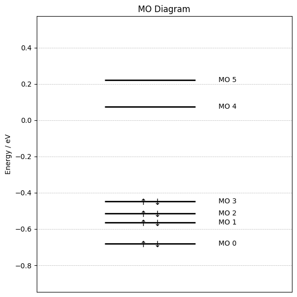
Plot a Molecular Orbital Diagram.
Visualize the Canonical Frontier Orbitals.
Visualize Localized Orbitals.
Step 1: Installing 3rd-party Dependencies
import sys
!{sys.executable} -m pip install --upgrade py3Dmol matplotlib
Step 1: Import Dependencies
We begin by importing all required Python modules for this tutorial. These include:
Note: We import modules for visualization/plotting like
py3Dmol. For this, it might be necessary to installpy3Dmolinto your OPIvenv(e.g., by activating the.venvand usinguv pip install py3Dmol).
# > Import file and directory handling
from pathlib import Path
import shutil

# > For advanced formatting in the notebook
from IPython.display import display, HTML
# > Import py3Dmol for 3D molecular visualization
import py3Dmol
# > Import matplotlib for plotting the MO diagram
import matplotlib.pyplot as plt

# > OPI imports for performing ORCA calculations and reading output
from opi.core import Calculator
from opi.input.structures.structure import Structure
from opi.input.simple_keywords import Sqm, Dft
from opi.output.core import Output
Step 2: Define Working Directory
All actual calculations will be performed in a subfolder moplot.
# > Calculation is performed in `moplot`
working_dir = Path("moplot")
# > The `working_dir`is automatically (re-)created
shutil.rmtree(working_dir, ignore_errors=True)
working_dir.mkdir()
# > Small resolution for cube files to keep the notebook light.
# > When you run the notebook you can choose larger values like 80 for smoother plots.
resolution = 20
Step 3: Water Molecule for the Calculation
We define an input file in the xyz format. The molecule can be replaced by any other neutral closed-shell molecule.
# > Define cartesian coordinates in angstrom as python string
# > This is water
xyz_data_water = """\
3

O      0.763468    0.595031   -0.044642
H      1.526939   -0.000000    0.000000
H      0.000000    0.000000    0.000000\n
"""

# > Alternatively, you can look for example at benzene
xyz_data_benzene = """\
12

C           -2.95158423642050        2.35836999822196        0.00212739782561
C           -4.14091557872368        1.64991032110004       -0.02391969791354
C           -1.74327014548301        1.68241626024842        0.01580886453943
H           -0.81519254019611        2.23525638004230        0.03613893725966
C           -4.12193886194957        0.26549013111527       -0.03633830745306
H           -5.08380703117622        2.17736970961569       -0.03458931904917
C           -2.91363281240151       -0.41045644578612       -0.02272181643407
H           -5.05002896510879       -0.28732892430873       -0.05668593056825
H           -2.96638917152996        3.43867643167804        0.01180502937775
C           -1.72429350123808        0.29800642953493        0.00337863588478
H           -2.89880723879466       -1.49076322175885       -0.03241213524154
H           -0.78140991697788       -0.22946706970293        0.01402834177239\n
"""

# > Select one of the structures - you can change this to benzene
xyz_data = xyz_data_water

# > Visualize the input structure
view = py3Dmol.view(width=400, height=400)
view.addModel(xyz_data, 'xyz')
view.setStyle({}, {'stick': {}, 'sphere': {'scale': 0.3}})
view.zoomTo()
view.show()

# > Write the input structure to a file
with open(working_dir / "struc.xyz","w") as f:
    f.write(xyz_data)
# > Read structure into object
structure = Structure.from_xyz(working_dir / "struc.xyz")
3Dmol.js failed to load for some reason. Please check your browser console for error messages.
Step 4: ORCA Calculation
We employ the semiempirical GFN2-xTB method for orbital generation to make this notebook fast. Since this is a semiempirical method, MOs can qualitatively be off from DFT calculations. So alternatively you might want to use DFT methods such as r²SCAN-3c.
# > Set up path for the structure
xyz_file = working_dir / "struc.xyz"

# > Create a Calculator object for ORCA input generation and execution
calc = Calculator(basename="job", working_dir=working_dir)

# > Load the molecular structure from XYZ file
structure = Structure.from_xyz(xyz_file)
calc.structure = structure

# > Add calculation keywords
calc.input.add_simple_keywords(
            Sqm.NATIVE_GFN2_XTB, # > Native GFN2-xTB
            #Dft.R2SCAN_3C       # > Alternatively DFT methods like r²SCAN-3c can be used
)

# > Request PIPEK-MEZEY localization. These will be stored in the .loc file.
calc.input.add_arbitrary_string("%loc\nLocMet PM\nend\n")

# > Write the ORCA input file
calc.write_input()
# > Run the ORCA calculation
print("Running ORCA calculation ...", end="")
calc.run()
print("   Done")

# > Get output and use it to create the gbw json output with config
output = calc.get_output()
status = output.terminated_normally()
if status:
    output.parse()
else:
    raise RuntimeError("ORCA did not terminate normally.")
Running ORCA calculation ... Done
Step 5: Plot MO Diagram
We start by plotting an MO diagram. Below we define a function for plotting the MO energy levels. For larger molecules or larger basis sets this function likely has to be adjusted.
def plot_mo_diagram(energies, occupations, title="MO Diagram"):
    fig, ax = plt.subplots(figsize=(6, 6))
    ax.set_title(title)
    ax.set_ylabel("Energy / eV")
    lumo_id = occupations.index(0)
    homo_energy = energies[lumo_id-1]
    lumo_energy = energies[lumo_id]

    prev_e = None
    max_x = 0
    for i, (e, occ) in enumerate(zip(energies, occupations)):
        if prev_e is not None and abs(e-prev_e) < 0.01:
            x += 2
        else:
            x = 0
        if x > max_x: max_x = x
        prev_e = e
        ax.hlines(e, x - 0.4, x + 0.4, color='k', linewidth=2)

        if occ == 2:
            ax.annotate("↑", (x, e), textcoords="offset points", xytext=(-10, -5), ha='center', fontsize=12)
            ax.annotate("↓", (x, e), textcoords="offset points", xytext=(10, -5), ha='center', fontsize=12)
        elif occ == 1:
            raise ValueError("This function does not support plotting of UHF type wavefunctions.")

        # MO index on the right, start counting at 0
        if e > homo_energy - 0.5 and e < lumo_energy + 0.5:
            label = f"MO {i}"
            ax.text(x + 0.6, e, label, va='center', fontsize=10)

    ax.set_xlim(-1, max_x+ 1.25)
    ax.set_ylim(homo_energy - 0.5, lumo_energy + 0.5)
    ax.set_xticks([])
    ax.grid(True, axis='y', linestyle='--', linewidth=0.5)
    plt.tight_layout()
    plt.show()
Now we obtain the MO data from the OPI output via the get_mos function and plot the MO diagramm with the function:
mo_list = output.get_mos()["mo"]
energies = [mo.orbitalenergy for mo in mo_list]
occupations = [mo.occupancy for mo in mo_list]
plot_mo_diagram(energies, occupations)
Step 6: Visualize Frontier MOs
We define a function for depicting the molecular orbitals. The cube output object is obtained from the plot_mos function and read by accessing the cube property. The following orbitals are plotted: HOMO-2, HOMO-1, and HOMO.
def visualize_mos(output: Output, plot_list: list[int], resolution: int, gbw_type: str):
    """Visualize a list of mo indices"""
    # > For nicely visualizing multiple MOs in this notebook we wrap
    # > py3Dmol viewers in html
    html_blocks = []

    for mo_index in plot_list:
        # > Obtain cube data of MO
        cube_output = output.plot_mo(mo_index, resolution=resolution, gbw_type=gbw_type)
        cube_data = cube_output.cube

        # Set up Py3Dmol viewer for cube data
        view = py3Dmol.view(width=250, height=250)
        view.addModel(xyz_data, "xyz")
        view.setStyle({'stick': {'radius': 0.1}, 'sphere': {'scale': 0.2}})
        view.addVolumetricData(cube_data, "cube", {"isoval": 0.005, "color": "blue", "opacity": 0.8})
        view.addVolumetricData(cube_data, "cube", {"isoval": -0.005, "color": "red", "opacity": 0.8})
        view.zoomTo()

        # > HTML formatting
        viewer_html = view._make_html()
        html = f"""
        <div style="display:inline-block; text-align:center; margin-right:10px;">
            <div><b>MO {mo_index}</b></div>
            {viewer_html}
        </div>
        """
        html_blocks.append(html)

    # Display all viewers with labels
    display(HTML(''.join(html_blocks)))

# > Plot orbitals
nel, _ = output.get_nelectrons()
homo_index = nel // 2 - 1
plot_list = [homo_index-2,homo_index-1,homo_index]
visualize_mos(output=output, plot_list=plot_list, resolution=resolution, gbw_type="gbw")
3Dmol.js failed to load for some reason. Please check your browser console for error messages.
3Dmol.js failed to load for some reason. Please check your browser console for error messages.
3Dmol.js failed to load for some reason. Please check your browser console for error messages.
The canonical orbitals are delocalized. MO 3 is the highest occupied orbital (HOMO) and represents a lone pair of \(\pi\)-symmetry.
Step 7: Visualize Localized Orbitals
Now we visualize the localized orbitals from the PM localization scheme:
visualize_mos(output=output, plot_list=plot_list, resolution=resolution, gbw_type="loc")
3Dmol.js failed to load for some reason. Please check your browser console for error messages.
3Dmol.js failed to load for some reason. Please check your browser console for error messages.
3Dmol.js failed to load for some reason. Please check your browser console for error messages.
The localized MOs (LMOs) are linear combination of the three canonical orbitals shown in the section before. MO 2 and MO 3 can be viewed as representations of the two O-H bonds in the Lewis structure with \(\sigma\)-symmetry, while MO 1 represents a lone pair of \(\sigma\)-symmetry.
Summary
In this notebook we demonstrated how to obtain cube data for molecular orbitals from OPI and how to plot the results using py3Dmol. The notebook can be downloaded and run locally. The molecule can be replaced with any other neutral closed-shell molecule (adjustments migh have to be made to the MO diagram plot function). Also, the level of theory can be adjusted to any SCF method natively implemented in ORCA.