View on GitHub

CovaLED Analysis

This tutorial demonstrates how to use ORCA together with the ORCA python interface (OPI) to perform a Local Energy Decomposition (LED) analysis to decompose the interaction energy of a non-covalent host-guest complex. The subsystems are decomposed into fragments bound by covalent bonds which is possible due to the CovaLED. Additionally, post-processing for the fragment-pairwise LED (fp-LED) is performed, which allows the decomposition of interaction energies in exclusively pair-wise contributions.

In this notebook we will:

1. Import the required python dependencies.

2. Define a working directory.

3. Set up a host–guest input structure for our calculation.

4. Run an LED calculation for the complete system.

5. Assign a host and a guest automatically.

6. Run the calculations for host and guest.

7. Perform post-processing for the standard LED.

8. Perform post-processing for the fp-LED.

9. Gather the results in pandas dataframes.

10. Visualize the LED interactions with heatmaps.

11. Interpretation of the results.

Step 1: Import Dependencies

We start by importing the modules needed for:

• Interfacing with ORCA input/output

• Numerical calculations and data handling

• Plotting results

Note: We additionally import modules for visualization/plotting like py3Dmol. For this, it might be necessary to install py3Dmol into your OPI venv (e.g., by activating the .venv and using uv pip install py3Dmol).

from pathlib import Path
import shutil
import copy

# > pandas and numpy for data handling
import pandas as pd
import numpy as np

# > OPI imports for performing ORCA calculations and reading output
from opi.core import Calculator
from opi.output.core import Output
from opi.input.simple_keywords import BasisSet, Dlpno, \
    Scf, AuxBasisSet, Approximation, Wft
from opi.input.blocks import BlockFrag
from opi.input.structures.structure import Structure
from opi.utils.units import AU_TO_KCAL

# > Imports for plotting results visualization of molecules
import matplotlib.pyplot as plt
import seaborn as sns
import py3Dmol

Step 2: Working Directory and Conversion Factor

We define a subfolder covaled_ethane in which the actual ORCA calculations will take place. Also, we define a conversion factor, since we want the resulting interaction energies in kcal/mol for better interpretability.

# > Calculation is performed in `covaled_ethane`
working_dir = Path("covaled_ethane")
# > The `working_dir`is automatically (re-)created
shutil.rmtree(working_dir, ignore_errors=True)
working_dir.mkdir()

Step 3: Setup the Input Structure

As an example, we will take a simple ethane dimer. The 3D structure in Cartesian coordinates is defined and visualized:

# > define cartesian coordinates as python string
xyz_data = """\
16

   C   -7.95601053588590      3.15195494946836      0.27839423386884
   H   -8.05179200418556      2.32105035333223      0.97643318840757
   H   -8.76671687926839      3.06907938063429     -0.44469508271450
   H   -8.10439460873783      4.07476211185951      0.83796813304307
   C   -6.59679579710356      3.13992001745864     -0.41129316526153
   H   -6.44433232188420      2.21634557454439     -0.96856734466103
   H   -5.78737090643299      3.22474156709677      0.31305681682191
   H   -6.50317719735328      3.96948543870281     -1.11109265496380
   C   -7.98491788051681     -0.47692316195123     -0.27920144845602
   H   -8.79547255792874     -0.40025515615629      0.44475840345098
   H   -8.14024532507479     -1.38893575993245     -0.85442072275227
   H   -8.07387099754762      0.36622931992467     -0.96327738147245
   C   -6.62637230870360     -0.48881716933962      0.41184856873533
   H   -6.54173070676907     -1.33138502402438      1.09714355762301
   H   -6.46548339397797      0.42323949114744      0.98551040416686
   H   -5.81650657862927     -0.56907193276525     -0.31256550583595\n
"""

# > Visualize the input structure
view = py3Dmol.view(width=400, height=400)
view.addModel(xyz_data, 'xyz')
view.setStyle({}, {'stick': {}, 'sphere': {'scale': 0.3}})
view.zoomTo()
view.show()

# > Read the structure into object
structure = Structure.from_xyz_block(xyz_data)

3Dmol.js failed to load for some reason. Please check your browser console for error messages.

Custom Fragment Data Definition

The fragment data is assigned by the autofragmentator in the initial LED calculation for the supersystem. Alternatively, fragments can be define below if UseCustomIDs is set to True. A complete fragments list (starting at 1) has to be supplied and complete frag_in_sub_one lists with the IDs of the fragments in the subsystems have to be given:

UseCustomIDs = False # Change to True and adjust fragments and frag_in_sub_one for custom IDs.
if UseCustomIDs:
    # > list with alternative fragment IDs for each atom - change these as required. Start counting at 1. 
    fragments = [1, 1, 1, 1, 1, 1, 1, 1, 2, 2, 2, 2, 3, 3, 3, 3]
    # > define fragments in subsystem. Start counting at 1.
    frag_in_sub_one = []
    # > Fragments in the first subsystem - do not forget to update this
    frag_in_sub_one.append([1])
    # > Fragments in the second subsystem - do not forget to update this
    frag_in_sub_one.append([2, 3])

    # > Generate frag_in_sub starting from 0 for LED post-processing
    frag_in_sub = [[x - 1 for x in frags] for frags in frag_in_sub_one]
else:
    fragments = None

Step 4: Run CovaLED for the Supramolecular System

First, we run an LED calculation with DLPNO-CCSD(T)/def2-SVP for the complete system using NORMALPNO and NORMALSCF settings. We choose the small basis set and only moderate PNO and SCF settings to keep the computational costs for this notebook small. Note that these settings are usually not sufficient for production runs. The fragments in the CovaLED calculation will automatically be detected by ORCA (each ethane molecule is divided into two CH₃ fragments making four in total), but can also manually be assigned. We define and run three helper functions: setup_calc, run_calc, and check_and_parse_output.

First, we set up the calculation with setup_calc:

def setup_calc(basename : str, working_dir: Path, structure: Structure,  fragments: list[int] | None = None, ncores: int = 4) -> Calculator:
    # > Set up a Calculator object, the basename for the ORCA calculation is set to LED
    calc = Calculator(basename=basename, working_dir=working_dir)
    # > Assign structure to calculator
    calc.structure = copy.deepcopy(structure)

    if fragments:
        for id, atom in zip(fragments,calc.structure.atoms):
            atom.fragment_id = id

    # > Define a simple keyword list for the ORCA calculation
    sk_list = [
    Wft.DLPNO_CCSD_T, # > Use DLPNO-CCSD(T)
    BasisSet.DEF2_SVP, # > Use the def2-SVP basis set
    AuxBasisSet.DEF2_SVP_C, # > Use the def2-svp/c auxiliary basis set
    AuxBasisSet.DEF2_J, # > Use the def2-svp/j auxiliary basis set
    Dlpno.NORMALPNO, # > normal PNO settings
    Scf.NORMALSCF, # > normal SCF settings
    Approximation.RIJCOSX, # > Use RIJCOSX
    Dlpno.LED, # > Make energy decomposition
    ]

    # use simple keywords in calculator
    calc.input.add_simple_keywords(*sk_list)

    # > If specific fragments are desired they can be assigned,
    # otherwise ORCA's autofragmentator will create them.
    calc.input.add_blocks(BlockFrag(storefrags=True,fragproc="FUNCTIONALGROUPS,EXTEND,CONNECTIVITY",dointerfragbonds=True))

    # Define number of CPUs for the calcualtion
    calc.input.ncores = ncores # > 4 CPUs for this ORCA run

    return calc

calc_supersystem = setup_calc("supersystem", working_dir=working_dir, structure=structure, fragments=fragments)

Then we run the calculation with run_calc and obtain the output:

def run_calc(calc: Calculator) -> Output:
    # > Write the ORCA input file
    calc.write_input()
    # > Run the ORCA calculation
    print("Running ORCA calculation ...", end="")
    calc.run()
    print("   Done")

    # > Get the output object
    output = calc.get_output()
    
    return output

output_supersystem = run_calc(calc_supersystem)

Running ORCA calculation ...   Done

The successful calculation has to be checked and parsed, which is done in check_and_parse_output:

def check_and_parse_output(output: Output):
    # > Check for proper termination of ORCA
    status = output.terminated_normally()
    if not status:
        # > ORCA did not terminate normally
        raise RuntimeError(f"ORCA did not terminate normally, see output file: {output.get_outfile()}")
    else:
        # > ORCA did terminate normally so we can parse the output
        output.parse()

    # Now check for convergence of the SCF
    if output.scf_converged():
        print("ORCA terminated normally and the SCF converged")
    else:
        raise RuntimeError("SCF DID NOT CONVERGE")
    
check_and_parse_output(output_supersystem)

ORCA terminated normally and the SCF converged

Step 5: Definition of Subsystems

Next, we extract the automatic generated fragments and define a host and a guest subsystem. In our example, the host and guest system is one ethane molecule with two fragments each.

# > Shortcut to the fragments data
frags = output_supersystem.results_properties.geometries[0].geometry.fragments
# > Obtain the number of fragments in the led (fragment numbering continuous)
nfrags = int(output_supersystem.results_properties.geometries[0].mdci_led.numoffragments)

# > list of fragment IDs from LED calculation of supersystem. Starts counting at 0
fragments = []
for index, value in enumerate(frags):
    frag_id = int(value[0])-1
    fragments.append(frag_id)

# > If no custom fragment IDs were given the autofragmentator is employed and the interaction is calculated
# > between the first two fragments and all the other fragments.
if not UseCustomIDs:
    # > Define a list of fragments in the subsystems
    frag_in_sub = [[] for _ in range(2)]
    for ifrag in range(nfrags):
        if ifrag <= 1: frag_in_sub[0].append(ifrag) # > First two fragment are the guest (first subsystem)
        if ifrag > 1: frag_in_sub[1].append(ifrag)  # > All other fragments are the host (second subsystem)

# > define a mapping function between actual fragment_ids and fragment_ids for the subsystem calculations
def create_mapping(lst) -> dict[int, int]:
    return {val: idx for idx, val in enumerate(sorted(set(lst)))}

# > Starts counting at 0 as required for the LED post-processing.
sub_fragments_map = []
# > First subsystem
sub_fragments_map.append(create_mapping(frag_in_sub[0]))
# > Second subsystem
sub_fragments_map.append(create_mapping(frag_in_sub[1]))

# > generate atoms in fragments list. Start counting at 0.
atoms_in_frags = []
atoms_in_frags.append([val for val in fragments if val in frag_in_sub[0]])
atoms_in_frags.append([val for val in fragments if val in frag_in_sub[1]])

# > generate atoms in subsystem list. Start counting at 0.
atoms_in_sub = []
atoms_in_sub.append([i for i, val in enumerate(fragments) if val in frag_in_sub[0]])
atoms_in_sub.append([i for i, val in enumerate(fragments) if val in frag_in_sub[1]])

# > structure with fragment IDs for visualization
fragment_structure = output_supersystem.get_structure()
# > Visualize the fragments 
print("Here, the fragment IDs are depicted:")
for atom in fragment_structure.atoms:
    x, y, z = atom.coordinates.coordinates
    view.addLabel(f"{atom.fragment_id}", {
        'position': {'x': x, 'y': y, 'z': z},
        'backgroundColor': 'black',
        'fontColor': 'white',
        'showBackground': True,
        'fontSize': 12
    })
view.show()

Here, the fragment IDs are depicted:

3Dmol.js failed to load for some reason. Please check your browser console for error messages.

Step 6: Run the Host and Guest Calculations

sub_outputs: list[Output] = []
# > Loop over subsystems (host and guest), obtain substructures, and perform calculations
for i in range(len(atoms_in_sub)):

    # > Use map to map the global fragment ID to the subsystem fragment ID
    sub_fragments = [sub_fragments_map[i][atom]+1 for atom in atoms_in_frags[i]]
    
    # > Prepare calculation for the subsystem 
    subsystem = i + 1
    sub_structure = calc_supersystem.structure.extract_substructure(atoms_in_sub[i])
    calc_subsystem = setup_calc(f"subsystem_{subsystem}", working_dir, sub_structure, sub_fragments)

    # > Run the calculation
    output_sub = run_calc(calc_subsystem)
    
    # > Check and parse the output
    check_and_parse_output(output_sub)

    # > Visualize the subsystem
    xyz_data = output_sub.get_structure(with_fragments=False).to_xyz_block()
    view_sub = py3Dmol.view(width=400, height=400)
    view_sub.addModel(xyz_data, 'xyz')
    view_sub.setStyle({}, {'stick': {}, 'sphere': {'scale': 0.3}})
    view_sub.zoomTo()
    print("Visualizing the guest:" if subsystem == 1 else "Visualizing the host:")
    view_sub.show()

    sub_outputs.append(output_sub)

Running ORCA calculation ...   Done
ORCA terminated normally and the SCF converged
Visualizing the guest:

3Dmol.js failed to load for some reason. Please check your browser console for error messages.

Running ORCA calculation ...   Done
ORCA terminated normally and the SCF converged
Visualizing the host:

3Dmol.js failed to load for some reason. Please check your browser console for error messages.

Step 7: Processing for Standard LED

Now, we perform the post-processing for the LED.

# > Shortcut to the LED data for the supersystem
led_data = output_supersystem.results_properties.geometries[0].mdci_led

# > Number of fragments
nfrags = int(output_supersystem.results_properties.geometries[0].mdci_led.numoffragments)

# > Define shortcuts to the CCSD(T) energies for the subsystems (host and guest)
sub_outputs_energy = []
sub_outputs_led = []
for output in sub_outputs:
    # > get the CCSD(T) energy
    sub_outputs_energy.append(output.get_energies()["MDCI(SD(T))"])
    sub_outputs_led.append(output.results_properties.geometries[0].mdci_led)

# > Define variables to store the LED data
LED_pairwise_Total = {}
LED_pairwise_Ref = {}
LED_pairwise_Corr = {}
LED_pairwise_Ref_Coulomb = {}
LED_pairwise_Ref_Exch = {}
LED_pairwise_Corr_Disp = {}

# > First, we collect the results from the supersystem LED calculation
for x in range(nfrags):
    for y in range(x + 1):
        pair = (x, y)
        E_tot = led_data.totint[x][y]
        E_ref = led_data.refint[x][y]
        E_corr = led_data.corrint[x][y]
        LED_pairwise_Ref[pair] = E_ref
        LED_pairwise_Corr[pair] = E_corr
        LED_pairwise_Total[pair] = E_tot
        if x != y:
            E_ref_elstat = led_data.electrostref[x][y]
            E_ref_exch = led_data.exchangeref[x][y]
            E_corr_disp = led_data.dispcontr[x][y] + led_data.dispweak[x][y]
            LED_pairwise_Ref_Coulomb[pair] = E_ref_elstat
            LED_pairwise_Ref_Exch[pair] = E_ref_exch
            LED_pairwise_Corr_Disp[pair] = E_corr_disp

# > Now, we substract the results from the subsystem LED calculations
for x in range(nfrags):
    for y in range(x + 1):
        pair = (x, y)
        E_ref = 0.
        E_corr = 0.
        foundPair = False
        # > Check if both fragments are the guest
        if x in frag_in_sub[0] and y in frag_in_sub[0]:
            foundPair = True
            # > map global to sub fragment ID
            x_map = sub_fragments_map[0][x]
            y_map = sub_fragments_map[0][y]
            if sub_outputs_led[0]: 
                E_ref = sub_outputs_led[0].refint[x_map][y_map]
                E_corr = sub_outputs_led[0].corrint[x_map][y_map]
                if x != y: 
                    E_ref_elstat = sub_outputs_led[0].electrostref[x_map][y_map]
                    E_ref_exch = sub_outputs_led[0].exchangeref[x_map][y_map]
                    E_corr_disp = sub_outputs_led[0].dispcontr[x_map][y_map] + sub_outputs_led[0].dispweak[x_map][y_map]
            else:
                E_ref = sub_outputs_energy[0].refenergy[0][0]
                E_corr = sub_outputs_energy[0].correnergy[0][0]
        # > Check if both fragments are on the host
        elif x in frag_in_sub[1] and y in frag_in_sub[1]:
            foundPair = True
            # > map global to sub fragment ID
            x_map = sub_fragments_map[1][x]
            y_map = sub_fragments_map[1][y]
            if sub_outputs_led[1]:
                E_ref = sub_outputs_led[1].refint[x_map][y_map]
                E_corr = sub_outputs_led[1].corrint[x_map][y_map]
                if x != y and sub_outputs_led[1]:
                    E_ref_elstat = sub_outputs_led[1].electrostref[x_map][y_map]
                    E_ref_exch = sub_outputs_led[1].exchangeref[x_map][y_map]
                    E_corr_disp = sub_outputs_led[1].dispcontr[x_map][y_map] + sub_outputs_led[1].dispweak[x_map][y_map]
            else:
                E_ref = sub_outputs_energy[1].refenergy[0][0]
                E_corr = sub_outputs_energy[1].correnergy[0][0]

        # > Subtract the calculated data from the subsystems
        if foundPair:
            LED_pairwise_Ref[pair] -= E_ref
            LED_pairwise_Corr[pair] -= E_corr
            LED_pairwise_Total[pair] -= (E_ref + E_corr)
            if x != y:
                LED_pairwise_Ref_Coulomb[pair] -= E_ref_elstat
                LED_pairwise_Ref_Exch[pair] -= E_ref_exch
                LED_pairwise_Corr_Disp[pair] -= E_corr_disp

Step 8: Processing for fp-CovaLED

Next, we use the CovaLED results and post-process them to fp-CovaLED results, where the interaction energy is decomposed into only pair-wise terms. We calculate the scaling factors from absolute values for better numerical stability. The scaling is done for the total energies and for the reference energies, while the correlations contributions are obtained from subtracting the reference energies from the total energies.

def fp_analysis_abs():
    for x in range(nfrags):
        for y in range(x):
            pairXY = (x,y)
            pairXX = (x,x)
            pairYY = (y,y)
            E_Total_XY_unscaled = LED_pairwise_Total[pairXY]
            dE_Total_X_unscaled = LED_pairwise_Total[pairXX]
            dE_Total_Y_unscaled = LED_pairwise_Total[pairYY]
            E_Ref_XY_unscaled = LED_pairwise_Ref[pairXY]
            dE_Ref_X_unscaled = LED_pairwise_Ref[pairXX]
            dE_Ref_Y_unscaled = LED_pairwise_Ref[pairYY]
            denom_X_Total = 0
            denom_Y_Total = 0
            denom_X_Ref = 0
            denom_Y_Ref = 0
            # > Calculate the denominator of the weights with absolute values
            for k in range(nfrags):
                minXK = min(x, k)
                maxXK = max(x, k)
                pairXK = (maxXK, minXK)
                E_Total_XK_unscaled = LED_pairwise_Total[pairXK]
                E_Ref_XK_unscaled = LED_pairwise_Ref[pairXK]
                if k != x:
                    denom_X_Total += abs(E_Total_XK_unscaled)
                    denom_X_Ref += abs(E_Ref_XK_unscaled)
                minYK = min(y, k)
                maxYK = max(y, k)
                pairYK = (maxYK, minYK)
                E_Total_YK_unscaled = LED_pairwise_Total[pairYK]
                E_Ref_YK_unscaled = LED_pairwise_Ref[pairYK]
                if k != y:
                    denom_Y_Total += abs(E_Total_YK_unscaled)
                    denom_Y_Ref += abs(E_Ref_YK_unscaled)
            scalingX_Total = dE_Total_X_unscaled / denom_X_Total
            scalingY_Total = dE_Total_Y_unscaled / denom_Y_Total
            scaling_Total = scalingX_Total + scalingY_Total
            scalingX_Ref = dE_Ref_X_unscaled / denom_X_Ref
            scalingY_Ref = dE_Ref_Y_unscaled / denom_Y_Ref
            scaling_Ref = scalingX_Ref + scalingY_Ref
            # > Take the absolute values of the interfragment contributions
            E_Total_XY_scaled = scaling_Total * abs(E_Total_XY_unscaled)
            E_Ref_XY_scaled = scaling_Ref * abs(E_Ref_XY_unscaled)
            E_Corr_XY_scaled = E_Total_XY_scaled - E_Ref_XY_scaled
            # > Calculate Elprep contributions
            LED_pairwise_Ref_Elprep[pairXY] = E_Ref_XY_scaled
            LED_pairwise_Corr_Elprep[pairXY] = E_Corr_XY_scaled
            LED_pairwise_Total_Elprep[pairXY] = E_Total_XY_scaled
    
    # > Add the Elprep contributions
    for x in range(nfrags):
        for y in range(x):
            pairXY = (x, y)
            LED_pairwise_Ref[pairXY] += LED_pairwise_Ref_Elprep[pairXY]
            LED_pairwise_Corr[pairXY] += LED_pairwise_Corr_Elprep[pairXY]
            LED_pairwise_Total[pairXY] += LED_pairwise_Total_Elprep[pairXY]
    
    # > Set the intra-fragment contributions that were distributed to zero
    for x in range(nfrags):
        pair = (x,x)
        LED_pairwise_Total[pair] = 0.
        LED_pairwise_Ref[pair] = 0.
        LED_pairwise_Corr[pair] = 0.
        LED_pairwise_Ref_Coulomb[pair] = 0.
        LED_pairwise_Ref_Exch[pair] = 0.
        LED_pairwise_Corr_Disp[pair] = 0.

LED_pairwise_Total_Elprep = {}
LED_pairwise_Ref_Elprep = {}
LED_pairwise_Corr_Elprep = {}
# > Run the actual analysis
fp_analysis_abs()

Step 9: Gather the Results in pandas Dataframes

For easier access, we store the results in a dictonary of pandas dataframes.

# > Function for generating pandas dataframes
def gen_led_frame(led_dict: dict[tuple[int,int], float]) -> pd.DataFrame:
    # Create a full 2D array filled with NaNs
    grid = np.full((nfrags, nfrags), np.nan)

    # > Fill the grid with LED results
    for (x, y), value in led_dict.items():
        grid[y, x] = value * AU_TO_KCAL

    # > Convert to DataFrame
    df = pd.DataFrame(grid)
    # > Offset indices by 1 to start counting with 1
    df.index += 1
    df.columns += 1

    return df

# > Generation of data frames
data_frames = {}
data_frames["LED_Total"] = gen_led_frame(LED_pairwise_Total)
data_frames["LED_Corr"] = gen_led_frame(LED_pairwise_Corr)
data_frames["LED_Ref"] = gen_led_frame(LED_pairwise_Ref)
data_frames["LED_Ref_Coulomb"] = gen_led_frame(LED_pairwise_Ref_Coulomb)
data_frames["LED_Ref_Exch"] = gen_led_frame(LED_pairwise_Ref_Exch)
data_frames["LED_Corr_Disp"] = gen_led_frame(LED_pairwise_Corr_Disp)
data_frames["LED_Total_Elprep"] = gen_led_frame(LED_pairwise_Total_Elprep)
data_frames["LED_Ref_Elprep"] = gen_led_frame(LED_pairwise_Ref_Elprep)
data_frames["LED_Corr_Elprep"] = gen_led_frame(LED_pairwise_Corr_Elprep)

Step 10: Visualization of the Results in Heatmaps

Now we visualize the fp-LED total interaction energy in a heatmap:

# Function to plot the results in a heatmap
def plot_led(name: str, df: pd.DataFrame):
    plt.figure(figsize=(6, 5))
    sns.heatmap(df, annot=True,fmt=".1f", cmap="RdBu", center=0)
    plt.title(f"{name} (kcal/mol)")
    plt.xlabel("Fragment X")
    plt.ylabel("Fragment Y")
    plt.show()

# > Show the structure with fragment IDs once more
print("Visualization of fragments:")
view.show()

# > Calculate the total interaction energy between fragment 1 and everything else
etot = np.nansum(data_frames["LED_Total"].to_numpy())
print(f"Total interaction energy is {etot:.1f} kcal/mol")

# > Plot the heatmap
plot_led("LED_Total",data_frames["LED_Total"])

Visualization of fragments:

3Dmol.js failed to load for some reason. Please check your browser console for error messages.

Total interaction energy is -0.7 kcal/mol

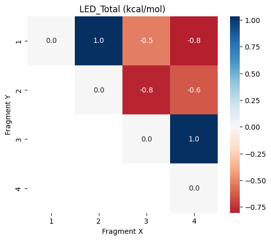
Step 11: Interpretation of the Results

The heatmap shown above visualizes the pair-wise contributions to the interaction energy of fragment 1 and the rest. The overall interaction energy is negative. We can also plot different contributions:

plot_led("LED_Ref",data_frames["LED_Ref"])
plot_led("LED_Corr",data_frames["LED_Corr"])

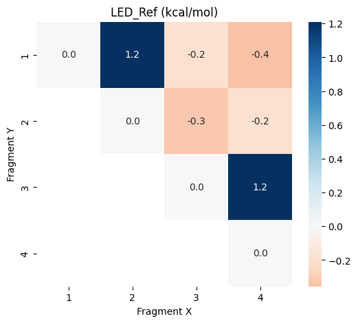
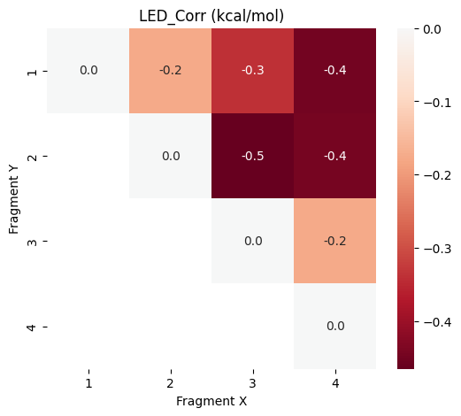
It can be seen that the correlation effects are critical for the overall negative interaction energy.

Note: If you are interested in the other contributions you can download this notebook, run it on your computer, and plot the other heatmaps with the functionality provided here.

Summary

The fp-CovaLED scheme was applied to an ethane dimer to showcase how to perform CovaLED calculations with the ORCA python interface (OPI). It is a helpful tool, e.g., for investigating protein–ligand interactions fragment-resolved. In principle, any structure can also be used with the autofragmentator, but care should be taken that no covalent bonds between the subsystems are broken.